A liquidity risk early warning indicator for Italian banks: a machine learning approach

This policy brief presents an early warning model to identify banks that could face liquidity crises, using a dataset built starting from those that resorted to the Emergency Liquidity Assistance (ELA). We applied three different models to estimate the probability for each bank to incur in a liquidity crisis: the logistic LASSO with blocked cross-validation, the random forest and the Extreme Gradient Boosting. Models’ signals have been calibrated through an optimization based on preferences between type I error (missing a crisis) and type II error (false alarm). To obtain a robust system, we then compared and combined the information produced by the three approaches. The three methods show an excellent predictive performance, which improves combining them through a simple or weighted average. The combined models achieve a low percentage of missed crises, while at the same time limiting the number of false alarms.

It is well-known and deeply studied in economic literature (e.g. Diamond and Dybvig, 1983) that creditors’ loss of confidence towards a bank can trigger a liquidity crisis, which could also cause difficulties to other financial institutions, threatening the overall stability of the system and adversely affecting the economy. To prevent contagion risks in the credit sector, central banks can intervene as a lender of last resort (LOLR). Providing Emergency Liquidity Assistance (ELA) represents the most traditional tool to contrast financial instability resulting from a liquidity crisis (BIS CGFS Papers, 2017; Dobler et al., 2016). ELA to financial institutions is a core responsibility of central banks because of their unique ability to create liquid assets in the form of central bank reserves, their central position within the payment system and their macroeconomic stabilization objective. To be able to intervene promptly or to adopt preemptive actions, central banks must have a set of methodological tools useful to anticipate the occurrence of these situations of instability. These tools are useful to attempt anticipating the need for liquidity support before formal action is required, so as to enable better information gathering and preparation. After the global financial crisis, central banks paid particular attention to developing or strengthening their early warning (EW) models.

In a recent paper (Drudi and Nobili, 2021), we developed an early-warning (EW) model to predict individual banks that could face a liquidity crisis. Unlike most of the literature, which focuses on the analysis of the insolvency risk and typically proposes a forecast horizon ranging from 4 to 6 quarters, we considered as the main forecast horizon the 3-month one. This choice depends on the fact that liquidity crises by their nature tend to arise quickly and require prompt intervention. Indeed, the choice of the forecast horizon has to satisfy the trade-off between being as short as possible in order to obtain very accurate estimates and being large enough to allow central banks to take corrective actions that could possibly avoid the onset of the crisis.

The EW model estimation is based on the interaction between a set of attributes, selected from those that can better signal the onset of potential crises, and a binary target variable that takes value 1 if a bank is going through a period of crisis and 0 otherwise. To construct this binary variable it is first of all necessary to identify which banks are facing a liquidity crisis. We decided to define our target variable in an extensive way by introducing an innovative dataset starting from banks that resorted to the central bank’s Emergency Liquidity Assistance (ELA). Considering only banks’ recourse to ELA, however, would be too narrow as ELA is only one of the possible outcome of a liquidity crisis. Moreover, banks’ recourse to ELA in Italy has not been frequent. For this reason, we extended the definition of liquidity crises to include other possible manifestations of banks’ liquidity deterioration.

Among other situations that arguably indicate a state of liquidity distress, we considered banks which have been subject to restrictive measures on participation to monetary policy operations and to enhanced liquidity monitoring by the Supervisory Authority. Finally, we also considered banks placed under special or temporary administration, subject to State support in the form of Government Guaranteed Bank Bonds (GGBBs) issues and deemed to be failing or likely to fail (FOLTF) for liquidity reasons.

As attributes, we considered 20 indicators selected in order to capture the peculiarities of the financing structure of Italian banks. These attributes are primarily liquidity and collateral indicators, but are also included capital ratios and NPL ratios and two variables related to the financial system as a whole.

Subsequently, we applied three different methods to estimate the probability for each bank to incur in a liquidity crisis in the following 3 months: the logistic LASSO with blocked cross-validation (Tibshirani, 1996), the random forest (Breiman, 2001) and the Extreme Gradient Boosting (Chen and Guestrin, 2016). The early warning literature usually presents the results coming from individual models. On the contrary, we aim at comparing and combining the information produced by the three approaches in order to obtain a more robust method for measuring banks vulnerabilities from a liquidity point of view. Indeed, it is likely that different approaches capture different linkages among variables that focus on specific types of fragility, and therefore can complement each other, giving value to their simultaneous use.

Moreover, following Sarlin (2013), we calibrated the signals of the models according to a loss function based on a policymaker’s preference between type I error (missing a crisis) and type II error (false alarm). The evaluation framework assumes that a central bank has to be substantially more concerned with missing a bank liquidity crisis than issuing false alarms. To take into account central bank’s preference for models that minimize type I error and in line with the majority of bank early warning literature (e.g. Betz et al., 2014, and Holopainen and Sarlin, 2017), for each method, the loss function has been optimized attributing a weight to missing a crisis far greater than the one of a false alarm. The rationale behind this choice follows the fact that an early warning signal should trigger actions by the authority to investigate and possibly restore the liquidity situation of the bank. Should the analysis reveal that the signal is false, there is no loss of credibility for the policymaker as model results are not published. Starting from the loss function, it is possible to compute two measures of usefulness that gauge the utility a policymaker can obtain from using a classification model with respect to not using it.

More precisely, once obtained the probabilities of incurring in a liquidity crisis in the subsequent 3 months for each estimation method, we optimized the loss function in order to get the optimal threshold. We considered the parameter of policymakers’ preferences between type I and II errors (μ) in a feasible range (μ ∈ (0.75, 0.98)), that corresponds to weighting a missing crisis between 3 and 49 times more compared to a false alarm. By comparing the probabilities of each estimation method with the different optimal thresholds, we defined the signals (0, 1) of the models.

Finally, we compared the goodness of the out-of-sample fit of the models through some performance measures based on the confusion matrix, which returns a representation of the statistical classification accuracy. Each column of the matrix represents the empirical crisis/ no crisis events, while each row represents crisis/ no crisis events predicted by the model (Table 1).

Table 1 – Confusion matrix

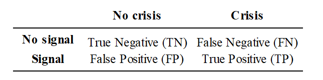
Table 2 shows the models’ out of sample evaluation measures when μ = 0.97, value that maximizes models’ relative usefulness. In addition to the usefulness and the relative usefulness computed through the loss function, Table 2 also reports the Accuracy, which computes the ratio of correctly classified observations over its total. Then, two measures of precision: precision positives and precision negatives. These ratios compute the percentage of model outcomes (signal/ no signal) that are correct. Finally, we add the false positive and false negative rates, which give a measure of how many times the model incorrectly classifies crisis cases or no crisis cases. As a comparison, we add in the table the evaluation measures also for the classical logistic regression. The results confirm that machine learning models perform better than the traditional logistic regression.

Table 2 – Models out of sample evaluation measures

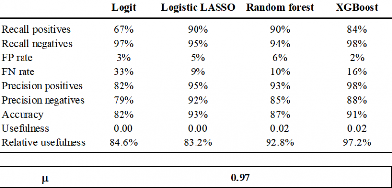
Note: The table reports the following measures to evaluate the performance of the models: TP FN Recall positives (o TP rate) = TP/(TP+FN), Recall negatives (o TN rate) = TN/(TN+FP), Precision positives = TP/(TP+FP), Precision negatives = TN/(TN+FN), Accuracy = (TP+TN)/ (TP+TN+FP+FN), FP rate = FP/(FP+TN) e FN rate = FN/(FN+TP).

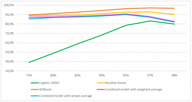
Changing the parameter of policymakers’ preferences between type I and II errors (μ) in the range μ ∈ (0.75, 0.98) leads to optimal results in line with the ones just presented. The relationship between the value of μ and the model relative usefulness is non-monotonic (Figure 1). As the value of μ increases, the model relative usefulness increases until reaching its maximum value and then it decreases again. For all the individual models the maximum relative usefulness is reached when μ = 0.97, whereas for the two combined models the maximum corresponds to μ = 0.95.

Figure 1 – Models’ relative usefulness changing μ

The key result of our paper is to show that complementing individual models improves the performance and yields to accurate out-of-sample predictions of bank liquidity crises (Table 3). In line with Holopainen and Sarlin (2017), we propose two different combination methods. The first one computes the combined probabilities as the simple average of the individual estimates. In this case, however, it is not possible to give greater weight to the model that has a better performance. To consider this, the second method weights the aggregation using the relative usefulness value of each model. In this way, the model with the best performance will provide a higher contribution to the output of the combined model.

The results show that the combined models manage to have an extremely low percentage of false negatives (missing crises) in out-of-sample estimates, equal to 10%, while at the same time limiting the number of false positives. These results are lower than the values usually reported in the literature. This could depend on our choice to test the model on a 3-month forecast horizon, which is perfectly suitable for liquidity risk models, but shorter than the horizon usually considered in insolvency risk models. In addition, in line with the results of Holopainen and Sarlin (2017), the weighted average model performs slightly better than the simple average one.

Table 3 – Combined models evaluation measures

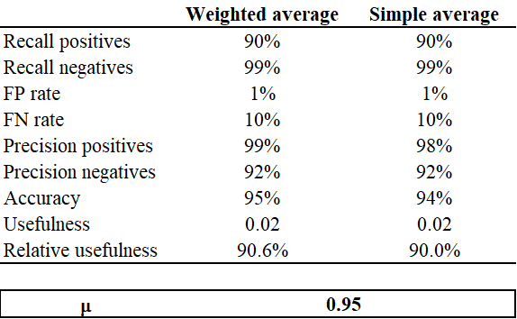
Note: The table reports the following measures to evaluate the performance of the models: TP FN Recall positives (o TP rate) = TP/(TP+FN), Recall negatives (o TN rate) = TN/(TN+FP), Precision positives = TP/(TP+FP), Precision negatives = TN/(TN+FN), Accuracy = (TP+TN)/ (TP+TN+FP+FN), FP rate = FP/(FP+TN) e FN rate = FN/(FN+TP). For the two combined approaches the maximum relative usefulness is reached when μ = 0.95.

To check the robustness of our results, we considered two further specifications of the target variable. The first one is based on a more restrictive definition of liquidity events. We considered only the events more closely linked to a liquidity deterioration such as resorting to central bank’s ELA, benefiting from State support through Government Guaranteed Bank Bonds (GGBBs) issues or, finally, being subject to enhanced liquidity monitoring by the Supervisory Authority. In the second robustness check, we considered as liquidity crisis event only the first month in which one of the events previously described occurred and excluded from the dataset the following observations related to that event for that bank. However, we allow for the possibility that during the period a bank incurs in different liquidity crises. Both specifications confirm that combining model probabilities allows improving the predictive performance, although the baseline specification results appear to be better.

Given the good predictive performance of our model, the signals obtained could become a useful tool for regular monitoring exercises, as they can help central banks to detect in advance banks that could be in need of central bank’s Emergency Liquidity Assistance (ELA).