
The COVID-19 pandemic represents a once-in-a-lifetime event, triggering an unprecedented policy response at the international level. The present paper draws from cutting edge economic, social and epidemic empirical literature and aims to offer policy-makers and researchers alike a wide set of quantitative tools to monitor the evolution of an epidemic curve in real time, to rank regions by epidemic risk, to assess the impact of restrictive measures and to uncover the relationship between viral spread, mobility and economic activity. Using a broad range of modelling techniques, from econometric to structural approaches, and combining them with qualitative approaches used in other areas such as financial stability dashboards, the holistic approach dives deep into analysing the COVID-19 pandemic for the case of Romania. To achieve these objectives we tackle several dimensions such as regional outbreaks and sub-epidemic waves, counterfactual scenarios based on structural frameworks and optimal lockdown policies, population mobility and initial considerations on the impact on economic activity.
The current pandemic caused by the SARS-CoV-2 virus presents the greatest challenge for public policy since World War II. The governments across the world have the challenging mission of managing this pandemic, as a result of the manifestly adverse effects on several levels: medical, economic and social. In this context, authorities need to find a mix of measures aimed at mitigating, in a balanced way, the medical effects of the new coronavirus while repositioning the economy on a path of sustainable growth. From an economic perspective, central banks play an essential role via the mandates and the objectives set by the legal framework. Central banks’ responses may differ significantly, depending on the economic, financial and epidemiological context of the country. It is therefore paramount to have a set of monitoring tools to gauge the epidemic spread that helps to adequately calibrate monetary and prudential instruments in order to achieve the fundamental objectives of maintaining price and financial stability.
Since the outbreak of the COVID-19 pandemic there has been a surge of empirical studies on modelling the epidemic curves and providing short-term forecasting or scenario analyses for policy-makers and researchers worldwide. Holmdahl et al. (2020) classify COVID-19 forecasting exercises in three main categories: (i) forecasting models, (ii) mechanistic models and (iii) hybrid approaches. The first category relies on statistical curve fitting to generate future expected values, without describing the underlying process leading to the realized values. Statistical tools, ranging from autoregressive and exponential/logistic growth models to machine learning techniques, can be implemented to produce accurate short-term forecasts (1-2 weeks), but are expected to be unreliable over longer time span. Mechanistic models have a structural foundation related to the transmission of the virus and can be used to simulate entire epidemic curves, as well as the impact of certain restrictive measures. Including information related to transmission, immunity and others in a Susceptible – Exposed – Infectious – Recovered (SEIR) framework (Kermack and McKendrick, 1927) together with feedback mechanisms allow researchers to produce long-term forecasts on the epidemic curves. Hybrid approaches draw inspiration from the empirical and theoretical advances registered in the medical, as well as statistical and technological fields, by combining the aforementioned categories of models to significantly improve on all the drawbacks that the naïve approaches exhibit. The Institute for Health Metrics and Evaluation (IHME) developed a complex hybrid model using a SEIR foundation and gathering a plethora of data on deaths, hospital utilization, social distancing and other measures. The model also accounts for mobility, testing per capita, mask effectiveness and usage, pneumonia seasonality and other aggravating factors. A similar extended SEIR framework is implemented by the European Centre for Disease Prevention and Control (ECDC) using Markov Chain Monte Carlo (MCMC) to build 30-day forecasts for all EU/EEA countries.
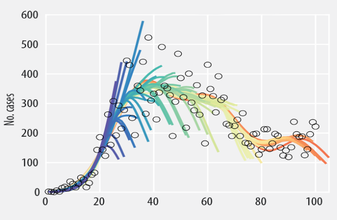
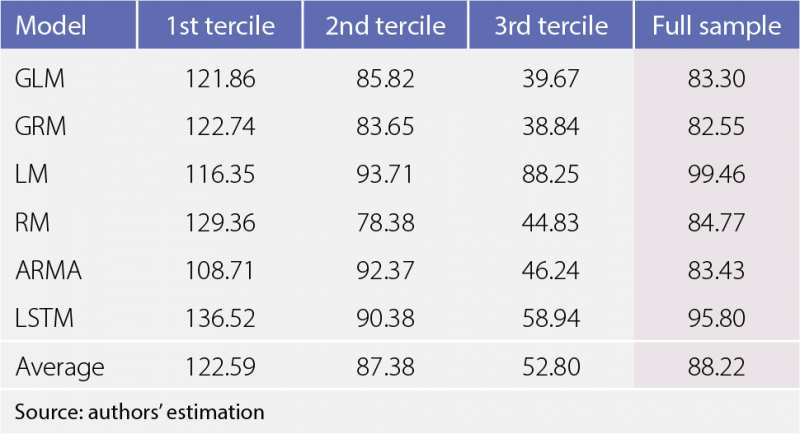
Taking into account empirically observed stylized facts related to COVID-19 epidemic waves worldwide, our toolbox employs a sub-epidemic modelling framework based on the idea that each epidemic curve is composed of several sub-epidemic waves, which allows for increased flexibility, including stable incidence patterns with sustained or damped oscillations and multi-modal curves due to structural factors such as seasonality, population density, mobility and others (Chowell, 2019). Complementary to the sub-epidemic framework which employs curve fitting models such as the Logistic and the Richards Model, a statistical approach, based on autoregressive models (ARMA), and a Machine Learning (Long Short-Term Memory approach) methodology are also considered to forecast epidemic dynamics on a short horizon of 10 days. As an empirical exercise we apply the forecasting methods on the first COVID-19 wave in Romania (March-June 2020); we find that for the first COVID-19 wave in Romania, the Generalized Richards Model (GRM) offers the best short-term forecasting performance (Figure 2.1), followed closely by the Generalised Logistic Model (GLM) and the statistical ARMA approach (Table 2.1). The results also highlight that introducing the possibility for asymmetry in the epidemic sub-waves increases forecasting performance, hinting at the idea of a slower decline rate once the peak of the epidemic wave has been reached.
| Figure 2.1. Iterative forecasting results for the Generalized Richards Model (GRM) | Table 2.1. Forecasting exercise performance (RMSE) for the epidemic and statistical models | |
 |
 |
|
| Note: Coloured lines represent iterative forecasting curves for each model, from dark blue to red, indicating the length of the data used for estimation. Empty circles denote the realized daily values. | Relative forecasting performance is assessed using the Root Mean Squared Error (RMSE) indicator, where a lower value indicates a better fit, computed for each forecasting iteration and taking average values over several sample slices. |
Taking into account empirically observed stylized facts related to COVID-19 epidemic waves worldwide, our toolbox employs a sub-epidemic modelling framework based on the idea that each epidemic curve is composed of several sub-epidemic waves, which allows for increased flexibility, including stable incidence patterns with sustained or damped oscillations and multi-modal curves due to structural factors such as seasonality, population density, mobility and others (Chowell, 2019). Complementary to the sub-epidemic framework which employs curve fitting models such as the Logistic and the Richards Model, a statistical approach, based on autoregressive models (ARMA), and a Machine Learning (Long Short-Term Memory approach) methodology are also considered to forecast epidemic dynamics on a short horizon of 10 days. As an empirical exercise we apply the forecasting methods on the first COVID-19 wave in Romania (March-June 2020); we find that for the first COVID-19 wave in Romania, the Generalized Richards Model (GRM) offers the best short-term forecasting performance (Figure 2.1), followed closely by the Generalised Logistic Model (GLM) and the statistical ARMA approach (Table 2.1). The results also highlight that introducing the possibility for asymmetry in the epidemic sub-waves increases forecasting performance, hinting at the idea of a slower decline rate once the peak of the epidemic wave has been reached.
Aggregating quantitative and qualitative data on pandemic dynamics − provided by indicators as well as modelling results, into an intuitive synthetic dashboard could provide a solution for clear communication and swift policy decisions. Dashboards usually contain a brief overview of the level (and outlook) of risks and vulnerabilities, via heatmaps or other ranking methods. Some recent eloquent examples are the European Systemic Risk Board’s Dashboard used for financial stability purposes, or the European Banking Authority’s Risk dashboard, part of the regular risk assessment done by this authority.
The PaMoD (Pandemic Monitoring Dashboard) is our first attempt at constructing a Dashboard for monitoring the COVID-19 pandemic (Figure 3.1). This preliminary exercise has been tested for the Romanian case and is meant to provide guidance for future research on this topic – each country could consider a tailor-made approach by combining information considered relevant by national authorities. The current approach contains 10 indicators grouped into three main categories, on a regional basis:
i) Epidemic potential – mainly focused on structural characteristics which can amplify the effects of the pandemic and lead to significant outbreaks in certain regions;
ii) Mobility – tracks population movement over the last 14 days as a proxy for the relative speed of the viral spread (various studies have shown a strong relationship between population mobility and epidemic curve dynamics);
iii) Epidemic curve – the indicators selected to track the dynamics of the epidemic curve are model-based, derived from GLM estimation, and used to assess the shape and profile of the epidemic wave.
The final step before aggregating individual indicators into scores for each category is represented by defining thresholds for the specific risk levels. As it would be difficult to find the optimal value for absolute thresholds, we resort to a relative risk ranking by computing percentiles of the distribution of each indicator.
Figure 3.1. A tentative structure for the Pandemic Monitoring Dashboard (PaMoD)
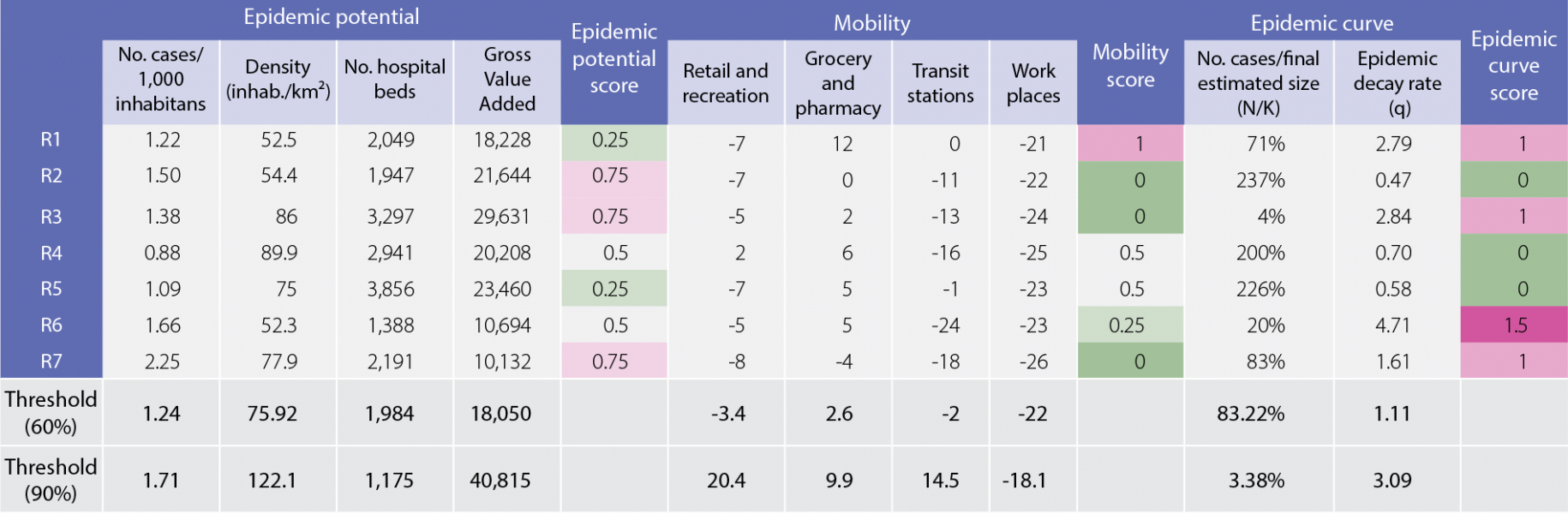
Note: Dashboard data were collected at the end of the first wave in Romania (June 2020). The aim is to provide guidance on how to build a Pandemic Monitoring Dashboard and not to draw conclusions on the medium-term epidemic developments in Romania. For adequate monitoring, the Dashboard needs to be updated frequently, as the conclusions can change significantly in a relatively low time frame. R1-R7 represent different regions (counties) for Romania.
Source: NIS, Eurostat, Google Mobility data, Romanian Ministry of Internal Affairs
We choose not to compute a final score due to the fact that each category highlights a different side of the epidemic risk, which renders the category scores non-additive from a policy perspective. For instance, having a higher epidemic potential does not directly imply a higher impact of the epidemic in that county, it just warns policy makers on certain structural vulnerabilities which can significantly amplify the effects of a potential outbreak.
In this section, we investigate the role that lockdown oriented policies have on the dynamics of the pandemic. To do this, our analysis has two components: investigating several ad-hoc scenarios regarding the implementation of lockdown scenarios and attaining an optimal lockdown policy. To achieve these objectives, we employ a benchmark Susceptible-Exposed-Infected-Recovered-Deceased (SEIRD) model.
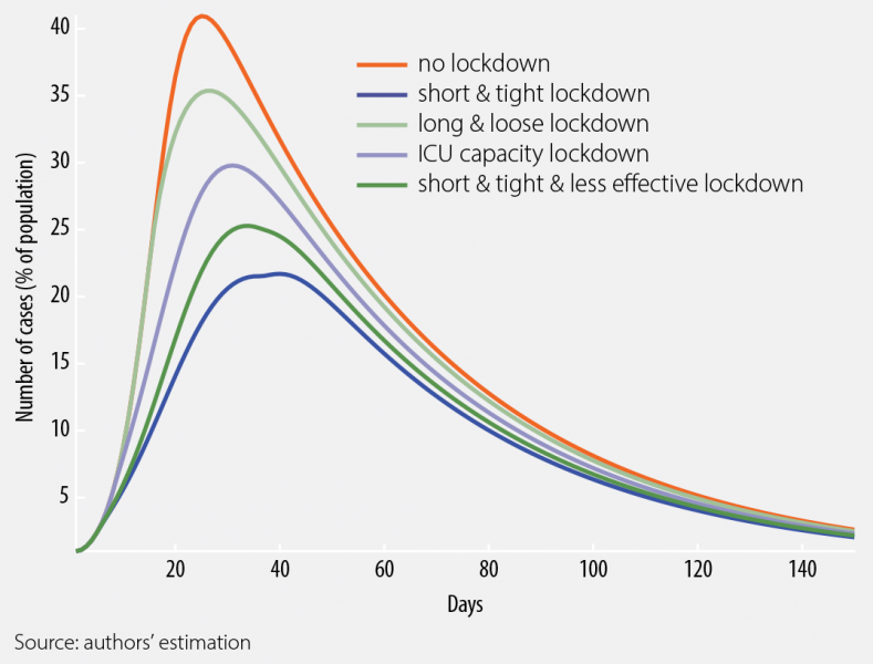
The lockdown scenarios defined in our work are designed as follows:
The results plotted in Figure 4.1 for the scenarios defined above firstly emphasize that: (i) all the considered lockdown measures are effective in reducing the number of new infections and (ii) the short and tight lockdowns are the most effective in reducing the virus spreading, while the long and loose lockdowns are not as effective in curbing the epidemic spread.
| Figure 4.1. Infection dynamics with the SEIRD model – fitting based parameters | Figure 4.2. Optimal lockdown and the related infection and recovery curves | |
 |
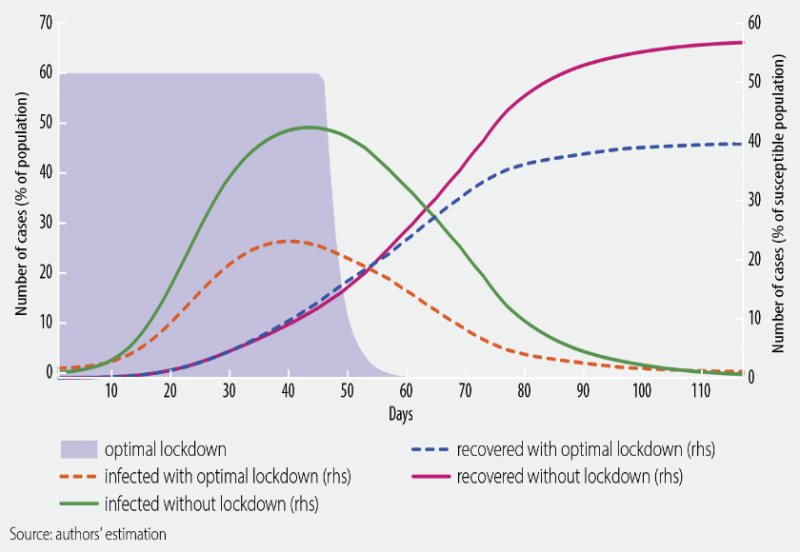 |
In the second part, we considered an optimal policy design defined as the lockdown setup that ensures the saving of most human lives while registering the lowest possible economic costs. Therefore, we ascertain that such a policy is Pareto optimal if there is no other possibility to save more lives and at the same time to have lower economic costs. In order to find such an optimal lockdown, we proceed by formulating an optimal control problem, with the lockdown being set as the control variable used to stabilize the situation in the medical sector, respectively in the economic sector. The objective function that we use here is very similar to the one in Alvarez et al. (2020), the difference being that we prefer a quadratic form for the lockdown design within the planner’s mandate. We employ this setup because we intended to exogenously take into account other different negative sides implied by the measures targeted at reducing the social distancing.
In the model calibration process, we consider a time interval of 120 days to approximate the length of the first epidemic wave for the case of Romania. We set the discount rate at 8% per year, the weight of the control is set in a standard manner to 1, while the other parameters are calibrated following the work of Acemoglu et al. (2020) and Alvarez et al. (2020). In figure 4.2 we report the resulted optimal control3, as well as the evolution of infected and recovered cases in the case of optimal lockdown, respectively with no lockdown. The results emphasize that the optimal lockdown policy has a very similar tightness degree compared to the short and tight lockdown designs and a duration similar to that of the loose and long controls. More precisely, the optimal control shows a tightness degree of 60% for approximately 50 days and, after that moment, the tightness degree decreases towards zero over the next 10 days. It is important to mention that the figures for the optimal lockdown and for the recovery and infection curves should be interpreted separately. While the lockdown is national, the infected and recovery curves refer to a pool that is susceptible to be infected by the first epidemic wave.
In a rapidly changing environment when, from day to day, the general conditions might be overridden, a simplified framework – that is able to provide very early signs about the severity as well as potential changes in the evolution of the epidemic and the economic situation – could be particularly useful. In order to build this framework, it is necessary to choose a few specific parameters that are able to capture the key characteristics of the coronavirus pandemic as well as the performance of the economy. Moreover, it is also important to find a link between the severity of the epidemic and its implicit economic costs. In this section, we first present a simple approach to monitor the evolution of the epidemic, then focus on the economic effects.
5.1. A simplified epidemic model
As the Corona crisis hit the economy and as the severity of the medical situation became the main driver of economic performance, experts have started to monitor an increasing number of indicators to keep pace with the latest developments, as well as to form a more comprehensive picture about the general conditions on the medical front. From this wide range of indicators, we select the effective reproduction number as the central element to include in our framework. The effective reproduction number, frequently denoted by Re or simply R, represents the average number of infections caused by a case of an infectious person in a population. In other words, R reflects how infectious the virus is and how quickly the epidemic spreads in a population. R(t) is a variation of this concept that captures fluctuation over time. In this section, we use R and R(t) interchangeably.
In order to stabilize the epidemic situation, it is necessary to reduce R to 1, while values below this threshold indicate that the epidemic wave is on its way towards fading out. A simple approximation of SARS-CoV-2’s effective reproduction indicator can be calculated as a ratio between the number of new daily registered infections on day t and its own 14-days rolling average (the latter is a proxy indicator for the evolution of active or infectious cases) at time t −1.
It is worth noting that, using this simple approach, the R indicator shows a delayed picture about the epidemic situation due to the incubation period (the time range from infection to the appearance of symptoms) as well as to the implementation of testing procedures. Therefore, when interpreting the trends, it is important to take into consideration the special effects coming from the lagging characteristic of observed data.
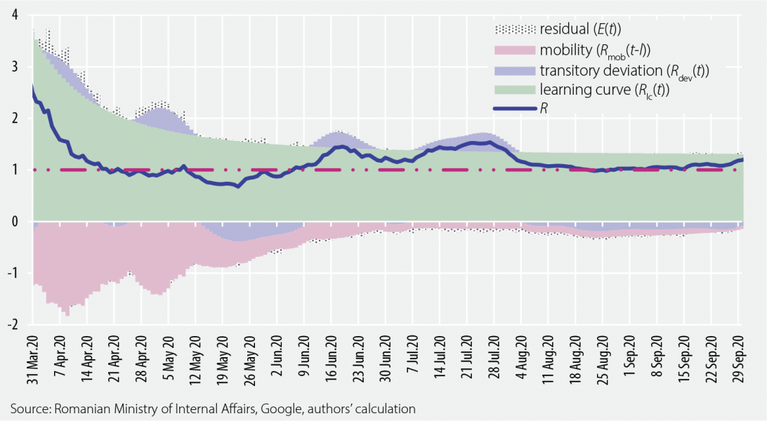
To form a deeper and more structured understanding about the drivers of the epidemic, we assume that R can be described as a by-product of three fundamental factors: (i) a non-observable learning curve Rlc(t), that determines the long-term evolution of the effective reproduction number; (ii) a cyclical process Rdev(t) allowing transitory deviations from the long-term trend Rlc(t), and (iii) the mobility level of households Rmob(t−l), a proxy indicator for the contact rate of individuals on day t−l. The l parameter captures the delay between infection and a positive test result. For technical reasons, an error term E(t) is also included in the analysis, so the final form of the equation becomes R(t)=Rlc(t) * Rdev(t) * Rmob(t−l) * E(t).
The fundamental explanation behind the learning curve Rlc(t) is that, at the outbreak of a new epidemic, R is expected to be significantly higher, as the society is facing a completely unknown virus. In the initial phase of the Corona-crisis, there was a complete lack of straightforward and detailed guidance on how to reduce the risk of infection. Moreover, sometimes, even contradictory information circulated in the public space. Over time, however, the society began to gather more information about the spreading mechanism of the SARS-CoV-2 virus and, accordingly, protection techniques were developed. Individuals became more conscious, trying to avoid personal contact, keeping adequate distance, wearing masks and so forth. Private economic agents as well as the public sector started to rapidly implement new approaches to reduce infection risk. Accordingly, the shape of the learning curve is downward sloping. In the long-run, the curve gradually flattens, approaching the threshold of 1. In other words, stabilising the epidemic through the learning process may require quite a long period of time. Of course, with very effective and large-scale vaccination, a scenario where the R indicator would fall below 1 on a sustained basis cannot be ruled out. In this case, the virus could disappear completely.
The second factor Rdev(t) might be interpreted as a series of waves around the learning curve Rlc(t) that are triggered by various reasons. Seasonality could be one such cause. At the moment, we do not have a complete understanding of the phenomenon. Nonetheless, there are signs suggesting that the evolution of the epidemic is influenced by seasonal factors. As in the case of influenza, the SARS-CoV-2 virus appears to spread somewhat slower during summer owing to warmer weather conditions, and faster in environments characterised by lower temperatures. Specific measures taken by authorities aiming to manage the epidemic situation, households’ loosening discipline and the appearance of local outbreaks may also trigger waves similar to those caused by weather conditions.
For a more comprehensive understanding of the impact of mobility Rmob(t−l), let us suppose the epidemiological wave is in a very early phase, therefore households’ mobility stays at pre-crisis level (Rmob(t− l) = 1) and the virus spreads particularly rapidly (e.g. R(t) = Rlc(t) * Rdev(t) * 1 = 2.2). In this situation, a significant reduction of households’ mobility would be able to slow the epidemic. If mobility decreases from 1 to only 0.4, ceteris paribus, the value of the effective R indicator is set to fall below the threshold of 1 (R(t) = Rlc(t) * Rdev(t) * 0.4 = 0.88). During the first epidemic wave, numerous economies of the world went through similar situations. After introducing countrywide social distancing measures in the second half of March 2020, the spread of the coronavirus slowed remarkably in April 2020. Later, as the reopening of the economy gained more traction, mobility had started to increase again in May-June 2020. As a result, R indicators across Europe pointed to a re-acceleration, yet the extremely high R levels seen in the spring outbreak were rarely reached due to the learning process Rlc(t).
Households’ mobility Rmob(t) was computed directly using data provided by tech giants. Unfortunately, the learning curve Rlc(t) and the cyclical component Rdev(t) are unobservable variables. Nonetheless, these can be approximated by applying trend estimation and filtering techniques frequently used in the case of GDP and other economic as well as financial time series.
Combining the three fundamental factors described above, we can decompose the evolution of the effective R indicator into its key drivers. Figure 5.1 shows the implementation of the model in the case of Romania (for the technical details please see Alupoaiei et al., 2021).
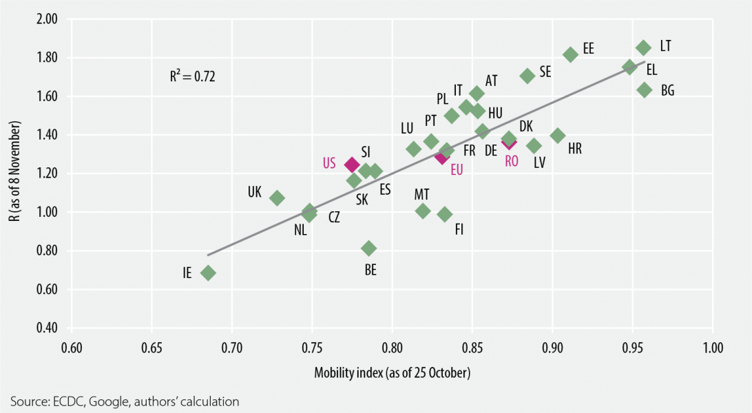
| Figure 5.1. Decomposition of the R indicator for the case of Romania (7-days moving average) | Figure 5.2. Cross country comparison of mobility and R indicators (14-days moving average) |
 |
 |
Note: the pre-crisis level of the mobility index is set to 1.
To analyse the evolution of the SARS-CoV-2 disease during the 2020 autumn wave as well as preparing in-depth cross-country comparisons are objectives going beyond the scope of this paper. Nonetheless, it is worth mentioning that, as weather conditions became colder, the transmission of the virus got impetus in Romania and, more generally, in Europe. With a short delay, the epidemic indicators worsened significantly in the United States as well.
Afterwards, in the period covering the end of October 2020 and the beginning of November 2020, the EU level R indicator marked a turning point. In this favourable evolution, the reintroduction of social distancing measures (translating to lower mobility) played a particularly important role. Statistics indicate that the spread of the epidemic slowed more in economies with low mobility levels (Figure 5.2). Although, among individual economies, significant variation can be detected owing to several country-specific reasons – country-level learning curves and cyclical deviations might be quite different –, data suggesting that reducing mobility near 0.75 (0.66-0.83) is sufficient to stabilise the epidemic situation. It is important to note that, in the case of the first wave, a much more drastic reduction, to around 0.40-0.50, was necessary to gain control over the spread of SARS-CoV-2.
In conclusion, the analyses suggest that although coronavirus is beatable, significant efforts are necessary to keep it under control. Meanwhile, the severity of the interventions should depend on how rapidly the disease spreads. Until vaccines or other efficient medical solutions become widely available, adjusting mobility level through individual decisions and/or public interventions remains one of the most powerful tools available for managing the health crisis.
5.2 Potential short-term costs of stabilising the epidemic
As discussed in the previous sections, the reduction of households’ mobility and, more generally, the contact rate of individuals are very effective tools in curbing the epidemic. Nevertheless, this solution could imply an exceptionally high negative impact on economic activity. In real-time, measuring precisely the effects seem to be a practically impossible challenge, as the costs may depend on a country’s economic structure, digital preparedness, integration level in global supply chains and a series of other specific factors. Nonetheless, in a simplified framework, it might be plausible to assume that a country’s economic activity level strongly depends on the evolution of nationwide mobility. In addition, when analysing really short time frames characterised by an epidemic outbreak, mobility Rmob(t) could be the most dominant factor of economic performance.
Nevertheless, official GDP estimates are published on a quarterly frequency and with substantial delays. Usually, the first estimate of real economic growth sees the light of day six weeks after the end of the reference period. Given these drawbacks, policy makers should use alternative indicators as well, to monitor, in a timely manner, the evolution of the economy amid adverse and rapidly changing conditions. For that purpose, we implement a dynamic factor model (DFM) to overcome these issues. The advantage of a DFM model is that it can exploit useful information from a wider set of monthly economic indicators. Moreover, the estimates of the DFM model are very easy to update following the release of new information. For a more detailed description of the DFM model as well as the full set of the explanatory variables, please see Alupoaiei et al. (2021).
In the following step, we compare mobility level with economic performance measured by DFM estimates as well as GDP to provide hints about the potential short-term economic costs of curbing the epidemic wave.
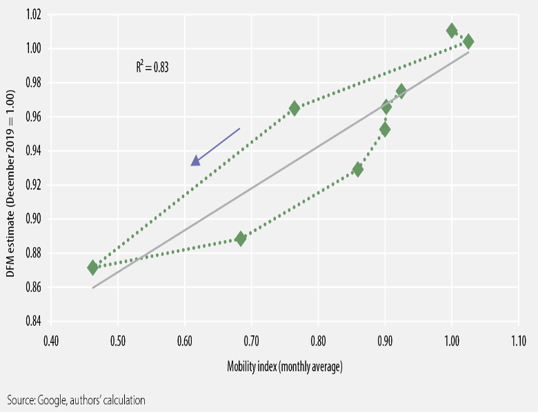
Unsurprisingly, there is a strong correlation between the level of mobility and the economic activity (Figure 5.3). More specifically, the analyses suggest that, in the case of Romania, a percentage point (pp.) drop in households’ mobility may drag down economic activity by around 0.25 (0.16-0.33) pps.
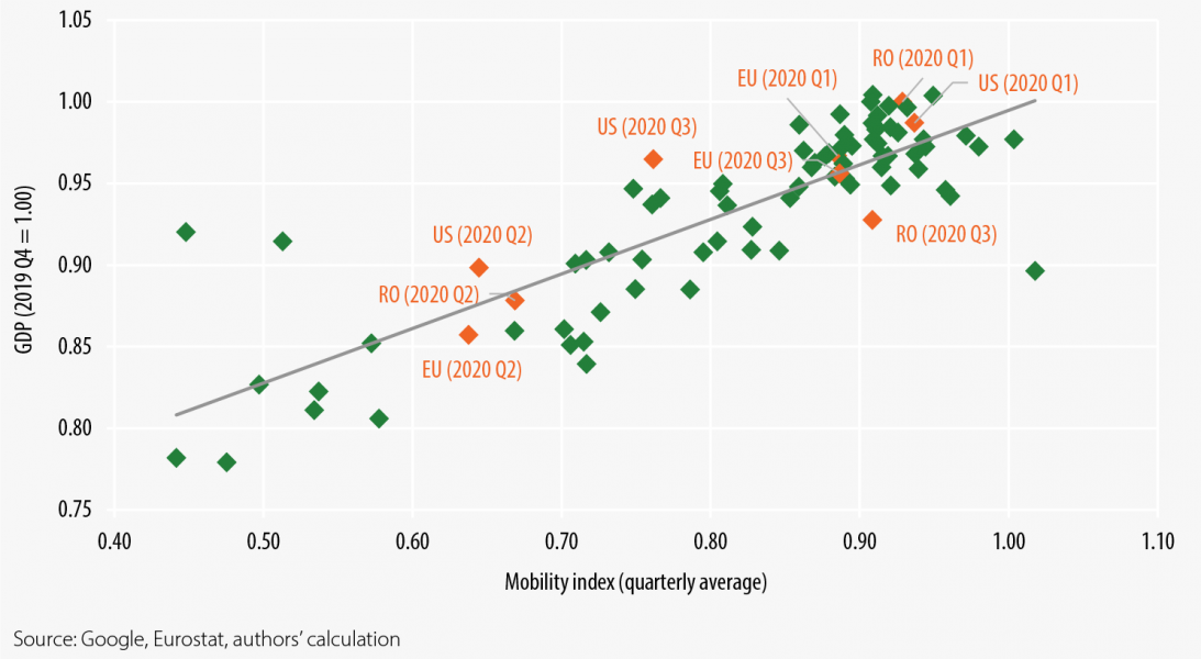
As previously noted, the evaluation of the relationships from a cross-country perspective is beyond the scope of this paper. However, using GDP data for the period of Q1 2020 – Q3 2020, we are able to extend our naï ve comparative analyses to the level of EU member states, the UK and US (Figure 5.4). In this regard, panel regressions in different setups – with or without specific cross section and period effects – point to quite similar results with coefficient estimates varying in the range of 0.18-0.37. As economic agents gradually adopt new solutions to overcome the challenges generated by the epidemic, it seems likely that the sensitivity of economic output to mobility will weaken over time. Therefore, looking forward, lower coefficient values might be more adequate, when evaluating the future impact of social distancing measures.
| Figure 5.3. Comparison of the mobility index with the level of economic activity (monthly data) | Figure 5.4. Cross country comparison of mobility indices with the level of GDP (quarterly data) |
 |
 |
Note: the pre-crisis level of the mobility index is set to 1.
Concluding, although results obtained on a very short time period should be used cautiously, in a rapidly changing environment, our simplified framework may provide useful early signs, completing the wide range of in-depth and more structural evaluations carried out by policy-makers.
5.3 Economic costs simulations based on the values of statistical life (VSL)
Simulations regarding the lockdown setup clearly show that reducing population mobility leads to a significant decrease in the viral spread. At this stage of our work, we are interested to analyze the effects on the economic sectors based on the concept of the value of statistical life (VSL). This economic concept measures the magnitude of trade-offs between wealth (or income) and mortality risk. In order to gain insight into the aforementioned complex relationship, we use the approach of Hall et al. (2020) as it offers a closer connection with consumer behaviour. By doing this, we are able to determine the fraction of annual consumption that society is willing to sacrifice in order to save lives. In other words, the results show the value of lost lifetime years relative to the value of annual consumption.
For this purpose, we use the average between the 2019 computed VSL for Romania and the reported figures for the VSL in 2010. We consider a benchmark scenario where the risk aversion parameter was set to 5, while for the death probability we use the middle range for the figures reported by Hall et al. (2020) and we pick a value of 0.625%. As in Hall et al. (2020), we assume that the hypothetical life expectancy for COVID-19 casualties is 14.5 years. By applying the calibration described for the basic scenario, we obtain a fraction of around 34.53% of annual consumption that society is willing to sacrifice in order to save lives (Figure 5.5). It is important to underline that in the basic scenario, as in Hall et al. (2020), we choose a risk aversion parameter that is higher as compared to the usual calibration (between 1 and 3) within the general equilibrium models. Nevertheless, it is well known from the equilibrium asset pricing theory that higher values for the risk aversion, respectively for the subjective discount factor, have to be used in a non-general equilibrium framework to match the empirical data.
Figure 5.5. Economic costs (in percentage points of annual consumption) of COVID-19 pandemic
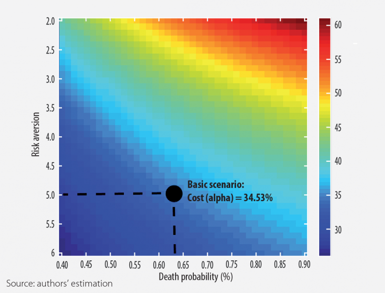
Note: the lifetime costs generated by fatalities are expressed in terms of annual consumption for a benchmark year.
Furthermore, we define several simultaneous scenarios for the probability of death, respectively for the risk aversion parameter. To ensure a granular approach, we use a range between 2 and 6 for the risk aversion, respectively between 0.4% and 0.9% for the probability of death. Looking at the results for various combinations of the parameters, we obtain a value of 25.97% for the fraction of the annual consumption that society is willing to sacrifice when the risk aversion is 6 and the death probability is 0.4%. Conversely, for a risk aversion of 2 and a death probability of 0.9%, the fraction of the annual consumptions that society is willing to sacrifice is 61.14 %. Summing up, the results underline the nonlinear relationship between death probability, risk aversion and the economic costs of COVID-19 pandemic fatalities.
Acemoglu, D., Chernozhukov, V., Werning, I. and M. Whinston, M. D. (2020), “Optimal Targeted Lockdowns in a Multi-Group SIR Model”, NBER Working Paper No. 27102.
Alupoaiei, A., Bálint, C., Kubinschi M. (2021), “A technical toolkit to monitor a pandemic outbreak from a central bank perspective”, NBR Occasional Papers No. 32. Available at https://www.bnr.ro/Occasional-papers-3217.aspx
Alvarez, F., Argente D. and F. Lippi. (2020), “A Simple Planning Problem for COVID-19 Lockdown”, NBER Working Paper No. 26981.
Barro, R. (2005), “Rare Events and The Equity Premium”, NBER Working Paper No. 11310.
Chowell, G., Tariq, A. and J.M. Hyman (2019), “A novel sub-epidemic modeling framework for short-term forecasting epidemic waves”, BMC Med 17, 164.
European Centre for Disease Prevention and Control (2020), “Projected baselines of COVID-19 in the EU/EEA and the UK for assessing the impact of de-escalation of measures”, ECDC: Stockholm, 2020.
Hall, R., Jones C., and P. Klenow (2020), “Trading Off Consumption and COVID-19 Deaths”, Working Paper, Stanford University.
IHME COVID-19 Forecasting Team (2020), “Modeling COVID-19 scenarios for the United States”, Nature Medicine, 23 October 2020.
Kermack, W. O., McKendrick, A. G. (1927), “A Contribution to the Mathematical Theory of Epidemics”. Proceedings of the Royal Society A. 115(772): 700–721.
This policy note is based on Alupoaiei, Bálint and Kubinschi (2021). The views expressed in this article are those of the authors and do not necessarily reflect those of the National Bank of Romania.
The tightness parameter takes values between 0 and 1, where 0 represents the case of no restrictions and 1 denotes a full lockdown scenario.
As in the first part of the analysis, the model is solved using the Runge-Kutta approach with adaptive step size, which we integrated within the Forward-Backward-Sweep method to obtain the optimal control.


