Can Machine Learning Methods Help Nowcast GDP?

Initial estimates of GDP are published with substantial delay. Nowcasting models aim to fill this gap and provide timely estimates of GDP. They can be used to provide estimates before the end of a quarter and quickly after the end of a quarter. Such models are now widely used in central banks and are typically based on dynamic factor models. An example is the nowcasting model of the New York Fed as described by Bok et al. (2018). Dynamic factor models explore a large number of time series to predict GDP. They extract a small number of factors that are common to these time series and use the factors to predict GDP.

In our paper with Dennis Kant (Kant et al., 2022), we compare the nowcasts of models that use alternative methods of aggregating the information from the large set of time series to the dynamic factor model of DNB. We use sparse methods that shrink coefficients in a large linear regression towards zero, such as LASSO and the elastic net, random subspace methods that use the power of forecast averaging, and the random forest that averages a large number of nonlinear regression trees.

The interpretation of the output of models with large number of input variables is challenging. The advantage of dynamic factor models is that they and the interpretation of the outcomes are well understood, see Banbura and Rünstler (2011). In particular, the output from the nonlinear random forest can be challenging to interpret, which limits its applicability in a policy environment. We use Shapley values to interpret the role of the different time series in the nowcast.

We apply these methods to Dutch GDP together with 83 macroeconomic and financial variables with monthly frequency. The data range from January 1985 to December 2018, and we use the period from January 1992 to December 2018 as our pseudo-out-of-sample forecast period. We produce backcasts, that is estimates of GDP produced after the quarter in question, nowcasts, which estimate GDP during the quarter, and short term forecasts up to two quarters ahead.

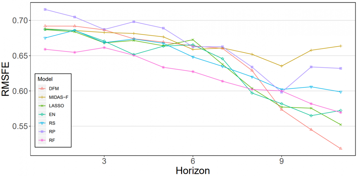
Figure 1 shows the root mean square forecast error (RMSFE) for the different horizons, where horizons one through three are two quarter ahead forecasts, horizons four through six are one step ahead forecast, horizons seven through nine are nowcasts, and horizons ten and eleven are backcasts. The first observation is that the RMSFEs shrink as more information becomes available, which implies that all methods successfully use the additional information that becomes available over time to improve the fore-, now- and backcast.

The figure also shows that the random forest is the most precise forecasting method until the first month of the quarter in question. In the middle of the quarter, the shrinkage methods, LASSO and elastic net and the random forest are roughly equivalent and the dynamic factor model is most precise for the last month of the nowcast quarter and for backcasting GDP.

Note: The figure shows the root mean square forecast error (RMSFE) of seven nowcasting methods for eleven monthly horizons. Horizons 1 through 3 are two quarter ahead forecasts, horizons 4 through 6 are one step ahead forecast, horizons 7 through 9 are nowcasts, and horizons 10 and 11 are backcasts. DFM: Dynamic factor model, MIDAS-F: MIDAS factor model: LASSO: Least absolute shrinkage and selection operator, EN: Elastic net, RS: Random subset regression, RP: Random projection regression, RF: Random Forest. Source: Figure 2 of Kant et al. (2022).

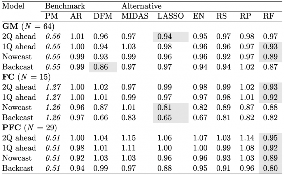
Table 1 reports the RMSFE relative to that of the prevailing mean benchmark over different sub-periods: The Great Moderation period from January 1992 to December 2007, the financial crisis from January 2008 to September 2011, and the period after the financial crisis from October 2011 to the end of the sample. Here, the horizons are aggregated to one-quarter, two quarter ahead forecast, nowcasts and backcasts. The shaded areas denote the most precise forecasts for a given horizon and period.

The table shows that, until and including the financial crisis, the dynamic factor model is largely eclipsed by other methods, in particular the random forest, for most horizons and periods. The difference is, however, small when it comes to nowcasting, which validates the popularity of the dynamic factor model. Since the financial crisis, however, the forecast accuracy has deteriorated and it is beaten by the random forest by a substantial margin. This is also true for all the other methods. It therefore appears that the nonlinearity of the random forest has become increasingly important since the financial crisis.

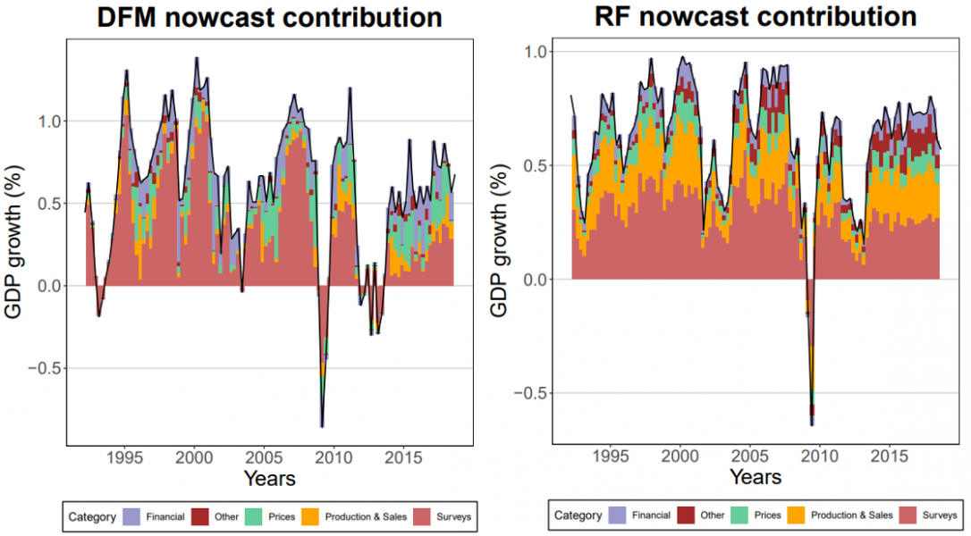
In order to shed light on the reasons why the random forest has outperformed the other models, We look at the contribution of the different subgroups of the data to the forecasts. Figure 2 reports the findings for the dynamic factor model and the random forest using Shapley values. Comparing the two plots, it becomes apparent that the random forest gives relatively more equal weight to the five different categories. Furthermore, unlike the dynamic factor model, the weight the categories were given did not change substantially since the financial crisis. The dynamic factor model gave very little weight to surveys after the financial crisis, despite this category having received the most of the weight prior to the financial crisis.

Note: The first column of the table gives the RMSFE of the prevailing mean (PM) model for different sub-periods in the pseudo-out-of-sample period. The following columns give the RMSFE of the respective nowcasting method relative to that of the PM.  A number smaller than one therefore indicates that the respective method is more precise than the prevailing mean. AR denotes the autoregressive model with lag length determined by AIC. For the remaining models see the footnote to Figure 1. GM denotes the Great Moderation, FC Financial crisis and PFM post financial crisis. In brackets are the number of observations per sub-period. Source: Table 3 of Kant et al. (2022).

Note: The bars show the relative part of the GDP estimates explained by a given category for the dynamic factor model on the left and the random forecast on the right. The black solid line represents the forecast of GDP by the respective method. Source: Figures 3 and 6 of Kant et al. (2022).

These findings suggest that, while the dynamic factor model is a competent nowcasting model, considering nonlinear alternative models, such as the random forest, can lead to improved nowcasting accuracy. Additionally, we also consider averaging the nowcasts of the different models, which provides nowcasts that are close to or as accurate as the best model and ensures against using a model with low accuracy.

References

Banbura, M., and G. Rünstler (2011) A look into the factor model black box: Publication lags and the role of hard and soft data in forecasting GDP. International Journal of Forecasting, 27: 333-346
Bok B., D. Caratelli, D. Giannone, A. Sbordone, and A. Tambalotti (2018) Macroeconomic nowcasting and forecasting with big data. Annual Review of Economics, 10: 615-643
Kant, D., A. Pick, and J. de Winter (2022) Nowcasting GDP using machine learning methods. DNB Working Paper 754
About the authors
Andreas Pick
Andreas Pick is associate professor at the Department of Econometrics, Erasmus University Rotterdam, and holds a part time position as researcher at De Nederlandsche Bank. Before joining Erasmus and DNB, he was a post-doc at the Economics Faculty in Cambridge and an Economist at the UK Debt Management Office. He has a PhD from the University of Cambridge.
Jasper de Winter
Jasper de Winter is principal economist in the Econometrics and Modeling Department, De Nederlandsche Bank. He has a PhD from Erasmus University Rotterdam.
More on these topics