menu
close

Author(s):

Juhana Hukkinen | Bank of Finland
Matti Viren | University of Turku

Keywords:

inflation , economic forecasts , inflation persistence

JEL Codes:

 Monetary Policy and Research department of Bank of Finland, and Monetary Policy and Research department of Bank of Finland & Economics Department of University of Turku, respectively. All opinions expressed here are our own and do not necessarily reflect those of Bank of Finland and the Eurosystem.

During the last two years we have regularly seen Christmas tree-shaped forecast profiles of inflation where the basic feature has been a rather quick return from high inflation to values close to the two per cent inflation target. Although this time-path is surely possible, historical data suggest that this kind of a “sudden stop” scenario is not very likely because high inflation rates seem to be more persistent and hence more long-living than commonly thought. Here we use IMF global data for 1970-2021 to show some key features of inflation developments, in particular probabilities of persistent inflation paths which make us think that the return to “old normal” may indeed take more time than what is generally assumed. 
Most economic forecasts predict that current high inflation is over in a couple of years, and in the end of 2024 we are back in the two per cent inflation regime (cf. e.g. IMF Outlook October 2022). But we have several reasons to doubt this consensus prediction (see e.g. Summers 2022 and Cochrane (2022) for discussion).
First, inflation is very persistent, at least when we have entered to the regime of two-digit inflation.  This shows up from a panel data of World countries. Thus, the first-order autocorrelation coefficient for inflation (computed from these data1) is 0.248 for the inflation regime between zero and four percent. But contrast, for inflation rates over four per cent and up to 100 percent, the corresponding value is 0.545 (for all positive values of inflation, the coefficient is 0.622).
Thus, there is not much movement from a low inflation regime to a high inflation regime and vice versa. That can be seen from the basic features of the data. In Figure 1, we have presented two subsamples of the global data: inflation rates for countries that have had the lagged moving average rate of inflation over 10 percent (upper curve) and countries that have (in the similar way) had inflation below 10 per cent. High past inflation clearly carries over to current inflation.
Figure 1: Inflation with high and low past inflation history 

 width=

Notes: Inflation history denotes 10-year lagged moving average of inflation. In the case of high inflation history, the values of the moving average values of inflation exceed 10 per cent. In the case low inflation history, the values are below 10 per cent. 
To obtain a bit more affirmative results, we have computed the probabilities of inflation staying above 4 per cent, or alternatively for being between 2 and 4 per cent and, finally, for getting negative values. These probabilities have been computed conditional to past inflation values which range from -5 to +30 per cent. The values that have computed with a five-year lag and are illustrated in Figure 2. Several other parametrizations and subsamples in terms of time were used but that did not make any qualitative change in results. Nor did the basic results change when Probit or Logit specifications were used.
Figure 2: Nature of continuing inflation 
 width=
Notes: Values are coefficient estimates from a linear probability model computed for 5-year lagged values of inflation (displayed at the x-axis as dummies for all rounded inflation rates) for three alternative cases. (a) inflation today is less than zero, (b) inflation is between 0 and 4, and (c) inflation is above 4 per cent. Here, the global panel data include 7445 data points for 1970-2021. 
The morale of the results is clear. If inflation has been over 5-6 per cent, it is highly probable that inflation continues to be above 4 per cent still after 5 years. By contrast, the probabilities of hitting values between 0 and 4 go down to 0.1 or less if inflation has been much higher. In practical terms, the probability of deflation goes to zero after the lagged inflation rate exceeds 10 per cent.
Alternatively. we can compute the probability of a big, say 5 per cent, decrease in inflation following various rates of previous year’s inflation (in the same way as in Figure 2). The results of this exercise are reported in Figure 3 again using coefficient estimates of a linear probability model.  Quite clearly, the probabilities are very low when inflation is below 10 per cent but after that the values increase even up to 50 per cent (reflecting the high volatility of high inflation2). But if we consider these big reductions in inflation rate, they seem to coincide with considerable reductions in GDP growth. In particular, the probability of depression clearly increases if inflation comes down by 5 percentage points or more.
Figure 3: Probability of a big fall in the inflation rate 
 width=
Notes: The displayed values are coefficient estimates of a linear probability model for all IMF countries for 1970-2021. N = 7869. The values on the x-axis are the inflation rates of the previous year. 
As a final exercise, we estimate a simple threshold model for lagged values of inflation, where we just have the first and second lag and allow all coefficient to change along with the (lagged) inflation regime. The regimes are determined on the basis of the sum of squared residuals criterion. A snapshot of the results is presented in Figure 4. They tell us that with low inflation (the estimated threshold being 1.8 per cent) past inflation does not matter much (only inflation two years ago has a marginal effect). But when we move to relatively high inflation regime (from 1.8 up to 15 per cent) things change dramatically. Inflation coefficients almost sum up to one suggesting that inflation becomes very persistent. But if we go even further (above 15 %) it is only the high constant term that matters both in terms of magnitude and significance. In other words, in the regime of very high inflation and inflation volatility, only the “sample mean” is focused on.
Figure 4: Threshold model coefficients for different inflation regimes 
 width=
Notes: The threshold is expressed in terms of lagged inflation. In the estimating equation, R2 = 0.47, N = 7905. Starred coefficient values are statistically significant (* = 0.05 and ** = 0.01). 
The above-presented results strongly suggest that if history repeats itself, we might have a much longer adjustment period towards the targeted values of inflation than what is generally perceived. It is true that in the historical data, there are high values of drops in the inflation rate, but they mainly coincide with the very high and volatile inflation periods. If we stick to the ten percent level of inflation, those rapid falls in inflation may not take place. The big danger in higher inflation is the fact that inflation is not only higher but also more persistent which makes anti-inflation policies more costly.

References

Cochrane, J. (2022) Inflation expectations. https://johnhcochrane.blogspot.com/2022/10/inflation-expectations.html
IMF Outlook (2022) https://www.imf.org/en/Publications/WEO/Issues/2022/10/11/world-economic-outlook-october-2022
Okun, A. (1971) The mirage of steady inflation, Brookings Papers on Economic Activity (2), 485–498. The Mirage of Steady Inflation (brookings.edu)

Summers, L. (2022) Twitter tweet on persistence of inflation on October 27, 2022. https://twitter.com/LHSummers/status/1585607005707931648


  • 1.

    All empirical analyses in this paper are based on global cross-country data on all IMF countries (193) for 1970-2021. Further details are available in our forthcoming discussion paper.

  • 2.

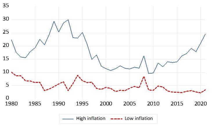
    When inflation is below 10 per cent, the sample standard deviation is 2.7 but if inflation is above 10 per cent (up 100 per cent), the standard deviation is already 17.4. This regularity was already pointed by Okun (1971).

About the authors

Juhana Hukkinen

Juhana Hukkinen is an advisor at the Bank of Finland. He has worked at the Bank of Finland since 1987. He made his studies at the University of Helsinki, first philosophy and then economics. Most of his work and research is related to monetary and fiscal policy and applied macroeconomic analysis.

Matti Viren

Matti Viren is professor of economics (emeritus) at the University of Turku and consultant at the Bank of Finland. Earlier he has served as a research supervisor at the Bank of Finland and as research director at the Government Institute of Economic Research. He has also been the Pre-accession advisor at the Polish Ministry of Finance in 2001-2003. He made his graduate studies at the Universities of Helsinki and Chicago and received his doctorate at University of Helsinki in 1980. Most of his research is related to economic policy and applied macroeconomic analysis.

More on these topics

Tags: