Devil is in the details: (mis)measurement of inflation

Recent inflation has been so extraordinary that even some long-forgotten issues of measurement have become relevant. Particularly pertinent are issues dealing with aggregation in an environment where inflation rates between different commodities and commodity groups differ significantly. In practice, this boils down to the weighting of different commodity groups. The problem is that weights are typically updated only annually, and even then, there are substantial lags. So, within a calendar year, constant weights are applied, which obviously causes bias in aggregate values because commodity-level inflation rates differ, and price elasticities also differ, resulting in a downward bias when inflation is accelerating and an upward bias when it is decelerating. In the Euro area, the bias surely existed in 2021-2023 but is outnumbered by the huge changes in consumption patterns caused by the Covid-19 pandemic.

How to aggregate micro-level inflation rates?

In the Euro Area, the aggregate price level is computed using the Laspeyres price index with fixed weights updated once a year. Therefore, with monthly data, the weight function becomes a step function that changes every January. While different countries may follow somewhat varied practices, it is generally safe to say that the January weights reflect, in most cases, household consumption behavior data that is at least 12 months old (see Box 1 below).

Box 1: Eurostat Manual definition of weights
The weight reference year is the calendar year t−2, i.e. 2 years before the new basket comes into effect in January of year t. The reference year expenditure is defined by the expression as obtained from the national accounts (or another source such as a household budget survey or other data sources) for product i at the weight reference year t−2. The expenditure data used should aim to be representative of year t−1 household consumption patterns. However, t−2 data are used as it is very unlikely that actual expenditure data for period t−1 would be available intime to be included in an index that will be reweighted to the month of January immediately following year t−1. In practice, expenditure from period t−2 is used, as this is the most up-to-date information available for the weights. …. For elementary product group and elementary aggregate indices, i.e. level II described above, the requirement is that the weights should be no more than 7 years old. See Eurostat HICP Methodological manual 2018, p. 47 and Eurostat 2020.

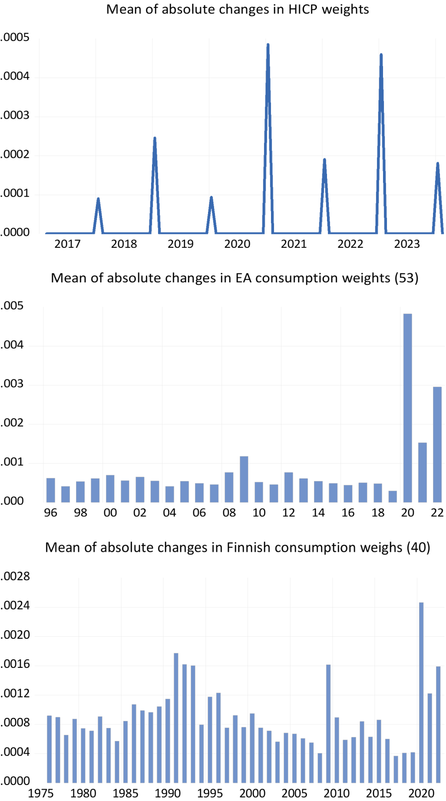
The magnitude of changes is illustrated in Figure 1 for the Harmonized Index of Consumer Prices (HICP) using our microdata of 280 commodities for the Euro area. For the sake of comparison, we also present (slightly more aggregated) changes in budget shares for National Accounts’ private consumption, both for the Euro area and for Finland. The HICP data cover the period from December 2016 to January 2024, the Euro Area National Accounts data span from 1995 to 2022, and the Finnish data cover the period from 1975 to 2022. It is evident that HICP weights represent lagged values of budget shares from private consumption. However, there are some puzzling values after the COVID-19 epidemic. In the private consumption data, but not in the HICP data, the COVID-19 peak is clearly dominating compared to the 2022 inflation peak (the 2023 values of HICP presumably mainly reflect the 2022 inflation peak).

Time lags are, of course, a practical problem that cannot be solved without a massive investment in data gathering and processing. A different, and potentially solvable, problem is related to the assumption that within the calendar year, the weight function remains constant. However, this would only be possible if the price elasticities were all unitary, which is not the case. For necessity-type goods like food, price elasticities are low. Therefore, when (relative) prices increase, their budget shares also increase. The problem might worsen if the prices of these goods increase more than goods with high price elasticity, as was seemingly the case in 2021-2023. Inflation rates were particularly high for food, heating, gasoline, and so on, while in most services, inflation rates were rather modest.1

Figure 1: Some data on changes in HICP & consumption weights

If we knew the price elasticities, we could, in principle, compute (and predict) the time path of budget shares. However, this is not easy due to the usual uncertainties regarding the size of the parameters, and especially because we lack information on the time horizon of elasticities. We are only aware of the long-run elasticities, not the short-run (‘monthly’) elasticities, except that, as a rule, they tend to be lower. Moreover, we would also need estimates of the cross-price elasticities. Even with these considerations, some simpler calculations can still be performed.

Assessing the magnitude of the possible bias

To provide a glimpse of the results, we present some outcomes using a simple moving average transformation of the official weight series instead of the straightforward step functions. The impact can be demonstrated through an example of tire prices shown in Figure 2. We applied the same procedure to all 280 commodity groups in our Euro Area microdata, forming the basis for HICP calculation (with the official weight series enabling exact recovery of the aggregate HICP price index). It is evident that moving average smoothing makes more sense in terms of inflation within the calendar year. However, the optimal solution would be to have budget share information available at least 6 months before the new year.

Figure 2: An example of the pattern of weights with EA micro data for tires

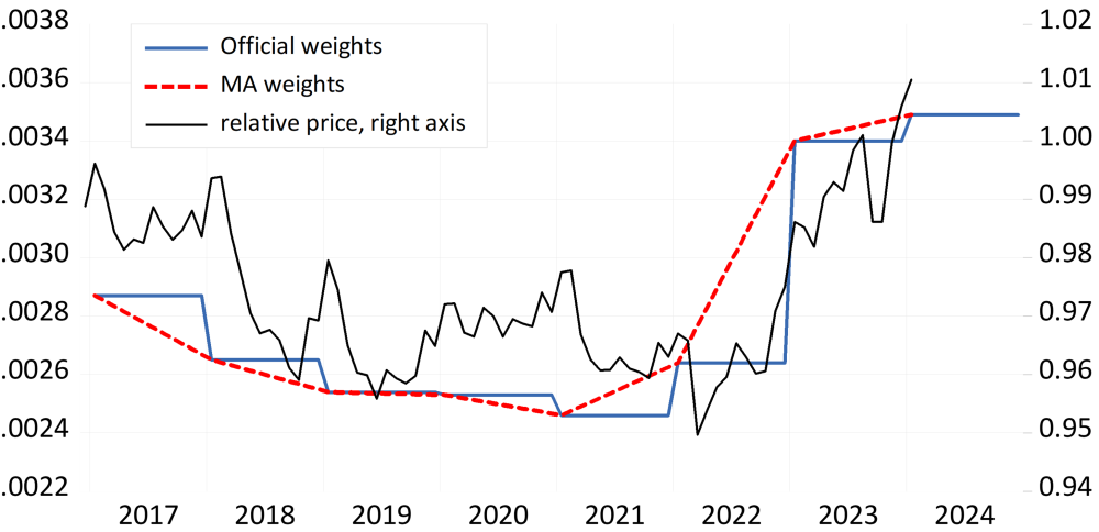
Figure 3: The effect of different weights on aggregate HICP inflation

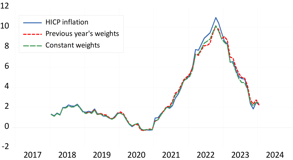
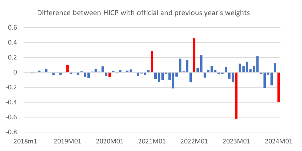
Nevertheless, even our simple calculations reveal that in 2022, the assumption of fixed weights for all months introduced some bias to the final estimate. The effect is however small compared with effects caused by the changes in the weights. In the later changes, the dominant effect was not the inflation-induced changes weights but the huge effects of the Convid-19 pandemic on consumption patterns. For instance, the budget share of food increased from 11.35 % to 13.03 % in 2020. Because these changes show up in the weights of HICP with a lag, the extraordinary budget shares affect the values of 2021 and 2022 causing the inflation rate to be much higher than if constant or lagged weights had been applied. The difference shows clearly in figure 3. In 2022 the annual difference is 0.6 per cent but in 2023 the bias changes its sign so that the value is about -0.3 per cent. The impact of weight changes can be seen from figure 4 where the official HICP one-month inflation rates are compared to the values where the weights represent the previous year’s official values. The new weights for January are indicated by red bars. Quite clearly, the changes in January deviate a lot from other months’ values.

Figure 4: The effect of updating new weights on HICP

Even though the Covid-19 pandemic makes all comparison difficult, it is evident that incorporating price elasticity values into the forecast of budget shares would add significant value. This is apparent from the estimated own-price elasticities shown in Figure 5. These elasticities represent a mixed bag, but nonetheless, they exhibit some systematic features similar to earlier empirical studies (e.g., Palmer 2019). Therefore, low elasticities are observed with necessity-type goods such as food and heating, which have recently contributed to inflation numbers. High inflation with necessities and their increasing budget shares evidently creates a complex situation, particularly for low-income households.

Estimates can also be derived from a simple double-log demand model where the log relative prices and log real income serve as the right-hand side variables. The values obtained are close to those obtained from the demand system(s).2 Only when the demand equations are estimated in first log differences do the demand elasticities become substantially lower, reducing the average value of 53 price elasticities to 0.499. The average income elasticities are consistently close to one.

Even if the average price elasticities are not far from one, we should not downplay the entire issue. Firstly, it is crucial to note that all elasticity estimates are essentially long-run estimates, and the more relevant short-run estimates can be much lower. On the other hand, a robust relationship between budget shares and past inflation is evident. As mentioned earlier, if the demand for all commodities is characterized by unitary price elasticity, the budget shares would not change in response to changes in relative prices. The clear contradiction to this assumption is revealed when running regressions between budget shares and inflation. It turns out that the relationship is clearly positive confirming that an increase (decrease) in relative prices increases (decreases) the budget shares in general. Casual evidence from the data also points in the same direction, as seen in Figure 6.

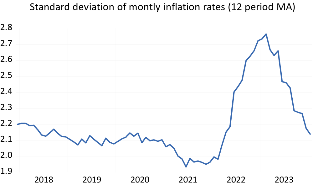
One might argue that forecasting budget shares is too challenging, but that does not necessarily have to be true. One indication supporting this notion is recent data suggesting that commodities lagging behind in terms of relative prices exhibit higher future inflation than commodities close to the average, not to mention those with high relative prices. Additionally, the dispersion of inflation rates (Figure 7) has proven to be a reliable predictor of future price changes. Note that it has not yet come to normal level, which is a bit alarming sign.

Figure 5: Estimates of own-price elasticities

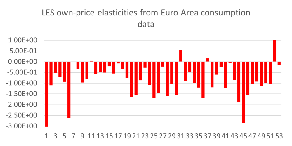
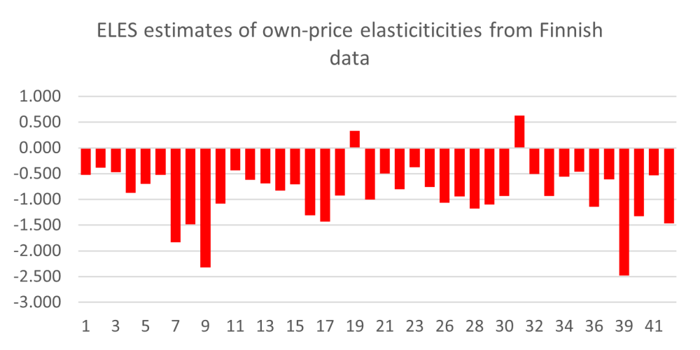
Note: The annual data for the euro area cover the period 1995-2022 and include 53 commodity groups. The Finnish data span from 1975 to 2022 and consist of 40 commodity groups. The numbers on the x-axis represent the code numbers assigned to these commodity groups. The mean values of the elasticities are 0.825 for the euro area (EA) and 0.871 for Finland. These estimates were derived using a linear expenditure system (see, e.g., Palmer (2019) and Clements et al. (2022)). The estimates are SUR estimates with robust t-values.

Figure 6: Relationship between commodity price changes and budget shares

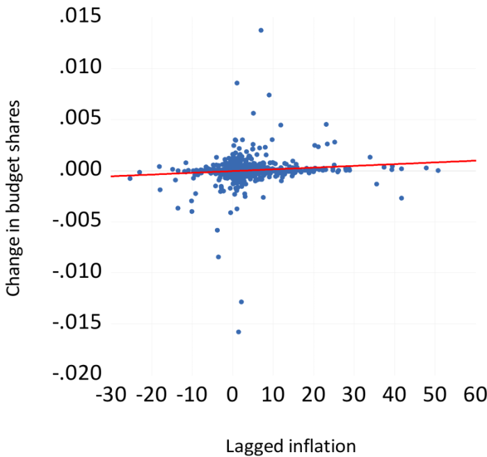
Figure 7: Dispersion of relative prices in the Euro Area

Concluding comments

Inflation has made a comeback to the set of important issues in macroeconomics. This compels us to pay closer attention to the empirical measures we employ in analytical work. This is particularly obvious in the aftermath of Covid-19 pandemic, which shocked the structure of consumption and consequently the weights of the price index in a profound way. However, the question at hand is not just about measurement. To comprehend the outcomes of different measurements, we need to apply at least the basic tools of consumer demand theory. With these tools, we might be able to produce more up-to-date data for economic analysis and for the general public. It is crucial to acknowledge that measurement outcomes are not merely ‘nice-to-know’ matters but carry significant implications for public policy, especially due to different indexing schemes.