menu
close

Author(s):

Juhana Hukkinen | Bank of Finland
Matti Viren | Bank of Finland

Keywords:

forecasting , financial markets , terms of trade , macro models

JEL Codes:

C52 , E27 , E37 , D8

All opinions expressed here are our own and do not necessarily reflect those of Bank of Finland or the Eurosystem.

During the recent surge of inflation from 2021 to 2023, a disappointing fact was the complete failure of forecasts to predict the coming storm. While nobody complains about the failures in predicting developments like 9/11 or COVID-19, it is commonly ignored that economists have been unable to predict practically all recessions and large booms. This observation clearly motivates discussion of the pitfalls of forecasting processes. In this paper, we argue that the main reason for these failures is the lack of use of financial market information, as well as an overreliance on a traditional national accounts framework in which the big picture of the economy’s growth potential easily fades away.

Why do forecasts fail?

Most economists probably agree that economic forecasts have not been very useful during the post-COVID-19 period, particularly in dealing with the recent surge of inflation from 2021 to 2023. However, it is not fair to say that this is the only episode when forecasts have failed. A paper by An et al. (2018) shows that, for the period from 1992 to 2014, practically all (148 out of 153) recessions came as a surprise. Even at the end of the recession year, a considerable share (one-fourth) of forecasts did not recognize that the economy was in a recession. A similar pattern was detected with economic booms.

These disappointing results clearly call for an explanation. While an exhaustive explanation cannot be provided, we can pinpoint some possible reasons for these failures. One such explanation is the model framework used in making forecasts. If we consider forecasts made by large institutions like central banks, ministries of finance, and international organizations, we must pay attention to the way different models are used.

Many institutions use sophisticated DSGE models to produce a theory-consistent set of values for all relevant macro variables. Even though this consistency is important, there are some obvious pitfalls in the procedure. First of all, the models use the national account framework, which, while definitely useful, is also rather restrictive in practical work. In this approach, it often happens that the general outcome is made in a “bottom-up” way by “summing up” the effects of different variables and sectors. Then it is not clear how the general economic “climate” is taken into account. This becomes more serious because typically we are just focusing on deviations from the steady path of the economy, but it is not at all clear how to differentiate these (cyclical) movements and the (steady state) trend growth. Finally, practically all models are built on the assumption of a representative household and firm. The latter assumption is clearly at variance with the data and is definitely not innocent in terms of productivity. In terms of future developments, the current average productivity growth can be much less important than the growth of the productivity frontier.

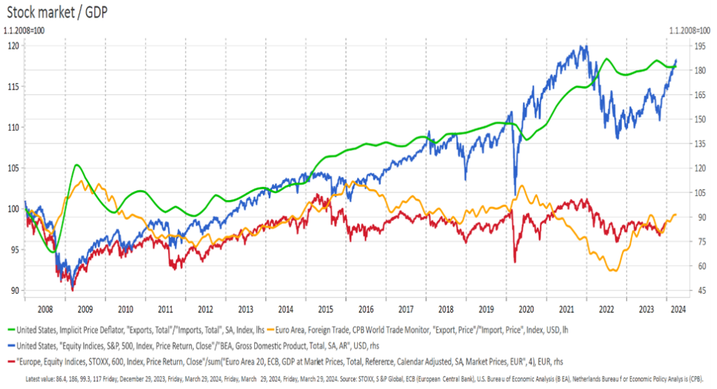
These considerations can be illustrated by comparing the financial developments of Europe (Euro area) and the USA (Figure 1), particularly during the post-financial crisis period from 2010 to 2024. Clearly, we see completely different developments in stock markets, terms of trade, exports, the term structure of interest rates, and so on. It is obvious that a typical DSGE model does not incorporate any elements that could account for these fundamental differences in economic development, which, of course, eventually show up in total production and different components of demand and income.

Figure 1. Fundamental differences between Europe and USA

In these (as well as other similar) models, technical change (or in statistical terms, total factor productivity) is either assumed to be constant or seen as an outcome of investment in R&D and/or human capital. However, if we focus on the biggest and fastest-growing U.S. firms, we have difficulties establishing a link between expensive R&D investments and the progress of these companies. Take, for instance, the list of the 10 biggest U.S. companies according to market cap values: Nvidia, Microsoft, Apple, Alphabet, Amazon, Meta, Berkshire Hathaway, Eli Lilly, Broadcom, and Tesla. In the case of medicine and semiconductor companies, the role of R&D is obvious. Otherwise, it is not at all clear that these companies owe their birth and growth to massive R&D investment.

This, in turn, means that predicting technical change with these often-cited background variables is not straightforward. This also suggests that models based on the National Accounts framework and a conventional production function may easily fail in the case of large supply-side shocks, irrespective of their exact content.

Building a model with the financial variables

These considerations motivate us to make forecasts based solely on the financial and technological drivers that determine the medium-term growth potential of the economy. In selecting these variables, we pay special attention to their importance in terms of the overall economic climate. When doing so, we strive to keep the model as parsimonious as possible, ensuring maximum transparency in the transmission mechanism and interpretation of outcomes. The respective variables are:
Stock prices:
The terms of trade
The term spread
Stock prices are expected to reflect the anticipated growth of corporate sector income. The simplest way to express this relationship is through the Gordon Growth Model. Additionally, stock prices are a key element of household wealth, which will ultimately translate into consumption growth in the future (see, e.g., Ball and French, 2021).
As for the terms of trade, it can be seen as a proxy for the “quality” of production and how advanced the exporting firms’ production is. This is reflected in the (relative) price of output and exports. It is no surprise that there is an ample amount of empirical research showing that the terms of trade is a key determinant of trade and economic growth (e.g., Wong, 2010). Here, we also briefly revisit some empirical evidence.
Finally, the term spread reflects the market’s expectation of future interest rates and economic conditions, with a larger spread indicating higher future interest and output growth rates. Previous analyses (e.g., Smets and Tsatsaronis, 1997; Ahmed and Chinn, 2023; and Minoiu et al., 2023) have established a strong relationship between the term spread and growth.
This approach to the forecasting problem is not new. In the past, there have been several attempts to replace detailed structural models with a simple reduced-form equation that relies on a handful of indicators without using the National Accounts framework. Perhaps the most notable example is the Friedman and Meiselman (1963) equation, which was later respecified and became known as the St. Louis equation by Anderson and Jordan (1968). The tracking behavior of this model, compared to the huge structural macro models of that time, created a lot of controversy, which was one reason for the dwindling popularity of these models in the 1970s and 1980s.

More recently, there has been growing interest in using various atheoretical models, either employing different time series model structures (like VAR) or models based on various forms of machine learning (e.g., neural networks). A common feature of these models is the use of a large number of high-frequency variables. This data allows consideration of many factors that are not present in the National Accounts setting, but it is typically impossible to trace back the reasons for a particular forecast outcome. Of course, that is not always necessary, but at least in policy work, it is clearly a negative feature. That is why we prefer a smaller model that can be opened up for closer scrutiny.

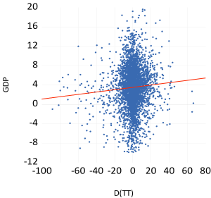
Before we focus on the results from our forecasting model, it is useful to scrutinize the key variables. We start with the terms of trade and GDP relationship. The basic nature of this relationship becomes apparent from Figure 2. The figure is based on data from 187 countries for the period 1990-2022, with 4004 observations. Clearly, there is a positive relationship between the terms of trade and GDP growth, which is also detected from panel data estimates, given different controls and fixed effects.

Figure 2. The terms of trade and GDP growth

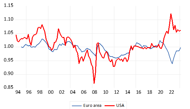
The role of the terms of trade may become more evident when we compare the behavior of the terms of trade indexes between the Euro area and the USA (Figure 3). By and large, the indexes moved similarly until around 2015, reflecting mainly the previous oil crises and the financial crisis of 2008-09. However, over the last 10 years or so, there has been a noticeable divergence: the US series has increased while the Euro area series has decreased, reflecting the diverging movements of stock prices (Figure 1). One might readily assume that this difference is due to the significant differences in the production and export portfolios of the largest companies in the Euro area and the USA. This divergence becomes more striking when comparing, for instance, the composition of the top 10 companies over time. In Europe, there is very little change in the ranking of companies, whereas in the USA, new tech companies have recently occupied the top positions. Needless to say, such changes are not reflected in National Accounts data, where the structure of production is less emphasized.

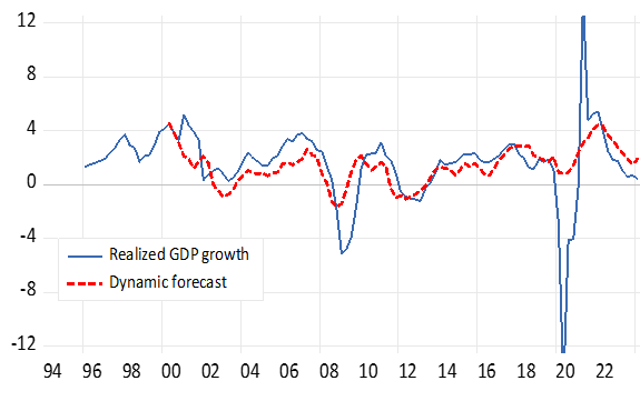
To determine whether these considerations matter, we estimate the basic equation with the aforementioned right-hand-side variables using data from Finland, Sweden, Germany, France, the UK, Italy, Spain, the Euro area, and the USA. In the basic specification, we use the Koyck lag structure. In all cases, the coefficients align with theory, although all estimates are not particularly precise. For example, we show a dynamic simulation path of quarterly GDP for the Euro area (Figure 4). While there are clear deviations from the data over time, the tracking record is reasonable given the length of the forecasting period. Needless to say, with shorter ex ante forecasting periods, the record improves significantly. Overall, the results suggest that even a very simple model can provide useful information about future movements in economic activity across different countries.

Figure 3. Comparison of terms of trade between EU and USA

Figure 4. Model simulation for the Euro area 1999-2024

Concluding remarks

Economic development in recent years has been marked by dramatic changes in technology, communication, and trade, which have profoundly affected productivity and competitiveness across different economies. It is also evident that these changes are not well captured by the current frameworks used to generate predictions for key macroeconomic variables. Therefore, it is worthwhile to focus more on models that reflect the key features of these developments. In general, this conclusion suggests that greater emphasis should be placed on various financial variables, changes in market shares, and the quality and relative prices of goods.

References

Ahmed, R. and M. Chinn (2023) Do Foreign Yield Curves Predict U.S. Recessions and GDP Growth? https://users.ssc.wisc.edu/~mchinn/foreign_yieldcurves.pdf.

An, Z., J. Jalles and P. Loungani (2018) How Well Do Economists Forecast Recessions? IM WP 18/39.

Andersen, L.& J. Jordan (1968) “Monetary and fiscal actions: a test of their relative importance in economic stabilization”, Federal Reserve Bank of St. Louis Review, 1968, 50, 11–24.

Ball, C. and J. French (2021) Exploring what stock markets tell us about GDP in theory and practice. Research in economics : an international review of economics, 75, 330-343.

Friedman, M. & D. Meiselman (1963) “The Relative Stability of Monetary Velocity and the Investment Multiplier in the United States, 1897-1958”, Stabilization Policies: A Series of Research Studies Prepared for the Commission on Money and Credit by E. C. Brown et al, Englewood Cliffs, NJ: Prentice-Hall: 1963, 165–268

Minoiu, C., Scchneider, A. and M. Wei (2023)  Why Does the Yield Curve Predict GDP Growth? The Role of Banks https://www.federalreserve.gov/econres/feds/why-does-the-yield-curve-predict-gdp-growth-the-role-of-banks.htm

Smets, F. and K. Tsatsaronis (1997) Why does the yield curve predict economic activity? Dissecting the evidence for Germany and the United States. BIS Working Paper 47.

Wong, H. (2010), “Terms of trade and economic growth in Japan and Korea: an empirical analysis”, Empirical Economics, Vol. 38(1), 139–158.

About the authors

Juhana Hukkinen

Juhana Hukkinen is an advisor at the Bank of Finland. He has worked at the Bank of Finland since 1987. He made his studies at the University of Helsinki, first philosophy and then economics. Most of his work and research is related to monetary and fiscal policy and applied macroeconomic analysis.

Matti Viren

Matti Viren is professor of economics (emeritus) at the University of Turku and consultant at the Bank of Finland. Earlier he has served as a research supervisor at the Bank of Finland and as research director at the Government Institute of Economic Research. He has also been the Pre-accession advisor at the Polish Ministry of Finance in  2001- 2003. He made his graduate studies at the Universities of Helsinki and Chicago and received his doctorate at University of Helsinki in 1980. Most of his research is related to economic policy and applied macroeconomic analysis.

More on these topics

Tags: