Does inflation come and go in the same way?

The failure to predict the surge in inflation in 2021 raises questions about whether we are better equipped to anticipate a future decline in inflation. What tools do we intend to use for predicting the trajectory of inflation? Are we still primarily relying on survey data regarding inflation expectations, and are we still employing a Calvo-type structure to model inflation, in which only the intensive margin (the size of price increases) adjusts in response to changes in demand and supply? We would like to emphasize that our highly disaggregated consumer price data for the Euro area, consisting of 280 commodity categories, strongly suggests that price increases (inflation) are influenced not only by aggregate trends but also by sector-specific developments that result in state-dependent price adjustments. These factors may lead to more volatile fluctuations in the inflation rate. Furthermore, these reactions do not appear to be entirely symmetric when it comes to rising and falling inflation. When the inflation rate is close to zero, the role of state-dependent pricing is diminished, and nonlinearities become less significant.

How to model inflation?

The recent failure to predict inflation necessitates a critical evaluation of the tools used to model inflation. One key tool in economic analysis is the New Keynesian Phillips curve, where inflation expectations play a central role. Inflation expectations are instrumental because of perceived price rigidities, which crucially affect pricing decisions. A common technical approach to modeling price rigidities is the Calvo-pricing scheme. This scheme assumes that prices can only be adjusted at specific points in time, with the probability of permission to change prices following a stochastic process with a constant frequency. In this setting, this frequency/probability serves as a “deep” parameter, meaning that changes in the inflation rate solely reflect changes in the size of price adjustments. Consequently, firms have access only to the intensive margin of pricing setting.1

While there has been some evidence supporting this setting, suggesting that the relative importance of intensive and extensive margin of price changes aligns with the data, it is now widely accepted that the extensive margin is not just important but often even more critical than the intensive margin. Therefore, in the current inflation landscape, the Calvo setting does not perform well, and this has significant policy implications.

Recently, Dunn et al. (2023), using UK Decision Maker Panel data, have shown that firms utilizing state-dependent pricing schemes have experienced noticeably higher price growth rates compared to those employing time-dependent pricing. This finding is further reinforced by Gautier and Le Bihan (2022) and Gautier et al. (2023), who demonstrate that the rapid transmission of large-scale shocks to prices is primarily due to changes in pricing behavior in response to these shocks.

There are several reasons for this skeptical attitude. First and foremost, we have witnessed significant shifts in commodity pricing due to the IT revolution. Menu costs associated with price changes have dramatically decreased, as evidenced by practices such as the so-called Amazon pricing schemes (Cavallo, 2022). Additionally, the nature of costs has evolved, leading to lower individual item pricing but increased costs related to the construction of pricing schemes, including the establishment of tolerance levels (Werning, 2023).

Another evident issue with pricing lies in the assumption that the probability of price changes does not align with the economic environment of a firm. Consequently, a firm that has refrained from altering its prices, falling behind its competitors, must patiently wait for permission to adjust its pricing. However, as pointed out by Golosov and Lucas (2007), this approach lacks practicality. It is suggested that instead of the Calvo scheme, we should consider adopting some form of state-dependent pricing.

Micro-level view of inflation developments

In this paper, we aim to address this issue by utilizing novel data from the Euro area, comprising 280 commodity groups. These data are derived from the fundamental information used to calculate inflation figures for the Euro area. They are reported on a monthly basis and cover a substantial period, dating back to the 1990s, though the complete dataset only spans from December 2016 to September 2023. Nevertheless, it contains a total of 23,800 observations. Consequently, these data exhibit distinctive micro data characteristics, allowing us to calculate relative prices and cross-sectional moments of the data.

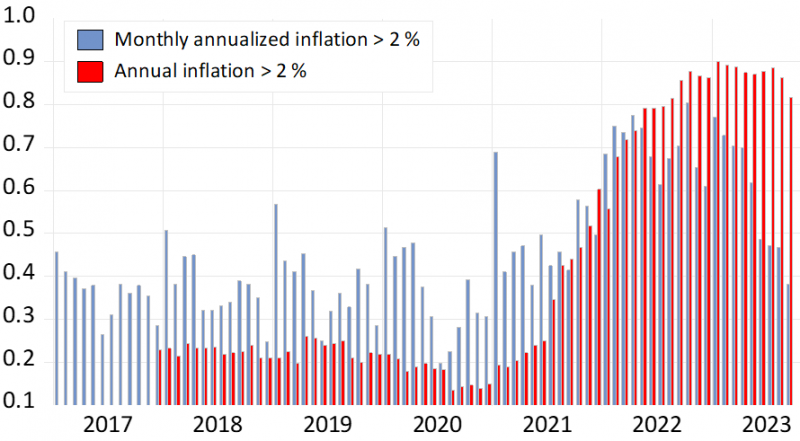
As a result, we can move away from the assumption of a representative firm and assess the implications of varying Calvo parameters for different commodities/firms. Figure 1 presents the key trends in recent inflation by examining the monthly changes in the price level averaged across these 280 commodity groups.

Evidently, the inflation pattern shows significant deviations when comparing the periods before and after 2021 (specifically, from January 2021). As inflation accelerated, it was primarily driven by the recent monthly price changes until April 2022, reaching its peak in October 2022. Subsequently, the monthly rates have consistently decreased. The 12-month change rate of the price level (annual inflation) responds to these developments with a substantial lag, with a clear turning point being observed only recently. Naturally, if we focus on thresholds other than 2 percent, these changes become more noticeable. So far, the monthly rate figures appear relatively symmetrical, suggesting that a rapid decline in high inflation is plausible.

Figure 1: Comparison of annual and monthly inflation

Essentially, a similar pattern emerges when we focus on measures of price level changes. Since commodity groups, such as group 280 (car tires), encompass numerous distinct commodities (brands), any change in the average price level for a commodity group registers as nonzero. As a result, we categorize an unchanged price level as one where the absolute monthly change rate is less than 0.05 percent or any similar threshold. Employing this threshold (or a comparable one), we generate Figure 2, which once again highlights an anomaly in 2021.

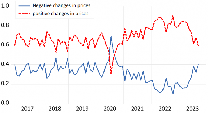
Prior to that, approximately 15 percent of prices remained unchanged, but after 2021, this figure dropped to around 5 percent. The current persistently high values can be attributed to an increasing number of price levels that are decreasing, which shows up in Figure 3. In 2022, up to 91 percent of prices increased, but by September 2023, this number had decreased to just 60 percent. It appears evident that only when annual inflation rates return to normal levels can we anticipate a return to the ’normal frequency’ of price changes seen prior to 2021.

Figure 2: Probability of a change in the price level

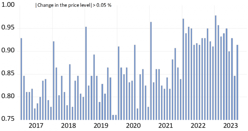
Figure 3: Shares of positive and negative price changes

State dependent pricing

Now, let’s shift our focus to the more significant aspect of state-dependent pricing. With our novel data, the intriguing question arises: Are current prices influenced not only by the (aggregate) market conditions but also by relative prices? One straightforward hypothesis is that if a firm is falling behind other firms in terms of pricing (i.e., it has not increased prices in a manner similar to its competitors), it has, all else being equal, an incentive to raise prices more than its peers. To investigate whether this hypothesis holds true, we conducted an estimation of a set of models using panel data. These models aim to predict current inflation by considering lagged inflation and lagged (log) relative prices (individual prices in relation to mean or median values).

Additionally, we included proxies to account for the range of relative prices and the standard deviation of inflation. These proxies were introduced to address the notion that as inflation increases, relative price differences tend to widen, subsequently increasing the necessity for price adjustments. This, in turn, affects the rate of inflation (or deflation).

Empirical analysis confirms these theoretical predictions. We have discovered a strong negative statistical relationship between relative prices and micro-level inflation. This association becomes even more robust when we incorporate fixed effects and seasonality as control factors.2 Therefore, when firms find themselves lagging behind the average price level, they tend to implement price increases more aggressively than firms that are either close to or above the average. This relationship holds true in the reverse scenario as well.

Notably, the significance of measures related to range (or volatility) adds further depth to the analysis. In periods of high inflation, the range of relative prices tends to expand, leading to a higher number of firms requiring price adjustments. The dominant feature here is the ’error-correction mechanism’ with a gradual return to the ’normal level’. However, it’s evident that this process may contain elements of ’overshooting’. Firms not only make necessary adjustments due to costs, such as real marginal costs, but also attempt to compensate for previous pricing errors. The broader the range of relative prices (or inflation), the greater the number of firms motivated by this compensation factor. The estimates consistently support this observation: the relative price effect is consistently negative, which leads to an error-correction type inflation effect.

Table 1: Relationship between inflation and relative price response

Note: Sample mean indicates the mean values of relative prices in the respective regime. Inflation effect is the respective contribution to inflation at the (sub)sample mean value. Thus, for instance in the first subsample regime, the sample mean shortfall in relative prices increases prices by 0.364 per cent in the next period. In estimation, all equations include a lagged standard deviation of relative prices and lagged inflation rates (up to 12 lags). The coefficient for the standard deviation of relative prices is always positive and statistically significant.

An intriguing question to explore is whether the adjustment follows a linear or nonlinear pattern, potentially influenced by specific menu cost characteristics. Our findings suggest that this is indeed the case. This outcome becomes evident when examining the results in Table 1 and Figure 4. Specifically, when we estimate a so-called threshold model, it becomes apparent that the relative price effect operates differently depending on the distance from the mean values of relative prices.

In this threshold model, the relative price effect is operational only when we are significantly away from the mean values of relative prices.3 The weight function (illustrated in Figure 4) of the smooth threshold model highlights the non-linear nature of the relative price effect. When we are close to zero of the logarithm of relative prices, the contribution of relative prices to inflation is practically negligible and not far from symmetrical (last column of Table 1).

Additionally, we found that the relative price effect is not operational when we are in the proximity of stable prices, specifically during the pre-2021 period. It appears that the effect (coefficient) becomes somewhat more pronounced with negative values of the logarithm of relative prices. This indicates that firms or industries lagging behind are more proactive in adjusting prices compared to those above the mean values. This can be interpreted as firms above the mean values being able to rectify the ’problem’ by not taking action, as inflation naturally facilitates the necessary adjustment, implying a longer adjustment period.

Figure 4: Smooth threshold weight function for the relative price effects

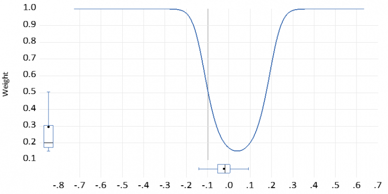
Note: x-axis = log of relative prices log(pi/P)t-1, the threshold parameters are here -0.095 and 0.171. The weight function reflects the same result as Table 1. Thus, when the price of commodity x does not deviate for the mean value, the relative price effect is close to zero and is not statistically significant. The more it deviates from the mean value, the stronger (significant) is the effect.

Some policy conclusions

There is a wealth of evidence indicating that a Calvo-type model does not provide a realistic representation of pricing dynamics. It tends to function effectively only in environments characterized by minimal or no inflation. However, when substantial shocks impact inflation, it becomes necessary to consider some form of state-dependent pricing, where pricing decisions are influenced by the dispersion of relative prices and firms’ pursuit of the optimal pricing strategy. This shift in perspective seems to result in more assertive pricing responses and a more volatile inflation profile. Clearly, the slow-moving survey expectations, along with the conventional New Keynesian Phillips curve, prove to be inadequate tools for the practical analysis of inflation in such circumstances, as emphasized by Cavallo et al. (2023).

The challenge we face is that even though there are indications of inflation ’normalizing,’ we cannot assume that the new normal mirrors the old normal. Several indications suggest that actual pricing behavior has undergone changes. We are witnessing the rise of more companies akin to Amazon, equipped with extensive data resources and fully computerized pricing systems. Additionally, there are innovations in the form of electronic price tags and a growth in sales that could revolutionize traditional retail practices. The recent surge in inflation may have acted as a catalyst for the emergence of new pricing technologies and a shifting pricing culture. These developments are likely to impact all relevant models and policy parameters in the future.