menu
close

Author(s):

Ernil Sabaj | Warwick University
Rashid Sbia | Aix-Marseille University
Haytem Troug | International Monetary Fund (IMF)

Keywords:

Fiscal multiplier , Government investment , Government consumption , Sectoral heterogeneity , Sector-specific shocks

JEL Codes:

E60 , E62

We study government spending multipliers in a panel of OECD countries. While recent literature has highlighted the differences in government consumption and investment effects, we extend this approach sectorally and report findings that suggest strong heterogeneities across sectors for government spending and output. Differences in price stickiness and sectors’ position in the production network are the main drivers of these heterogeneities.

1. Introduction

Government spending’s impact on the economy has been a subject of intense economic debate, especially after the recent financial crisis and the COVID-19 pandemic. Analyzing fiscal multipliers can provide insights into this matter. While prior research has focused on government multipliers’ heterogeneity across countries focusing on economic fundamentals; or the state dependency on the economy, recent studies have shifted the focus to the origins of the spending multiplier and the multisectoral effects of the economy. In addition, recent literature shows that there has been a significant focus on the US economy, while there is limited evidence available for other countries.
We contribute to the existing literature by estimating a panel VAR on selected OECD countries that focuses on the differences between government consumption and investment spending.1 We investigate these differences at the sectoral level, examining them from both a government and economic standpoint or combining both approaches. Furthermore, we offer an interesting perspective (usually neglected by the literature) by examining government spending according to the functions of the economy. The output multipliers that we calculated at the sectoral level vary from −1 to 1, depending on the type of government spending, whether it is consumption or investment, the sector in which the expenditure occurs, the function for which the spending happens, and the sector that the spending influences. We argue that these results are driven partially at the sectoral level by the differences in price stickiness across sectors and sectors’ positions in the production network. To our knowledge, this is the only paper that discusses these issues together.

2. Effects of sectoral government spending

In the first exercise (Fig. 1), we present the baseline panel VAR with results of a shock in general government spending, government consumption, and government investment2 by showing the responses in output, private consumption, private investment, trade balance, and the real effective exchange rate. The results show that a 1% increase in a general government spending shock causes a negative output response on impact. In contrast, the output response to a government investment shock is negligible. The estimated cumulative multipliers for the general government spending, government investment spending, and government consumption are respectively −0.46, −1.28, and 0.87. These results suggest that only government consumption can positively influence economic activity, private consumption, and private investment.3 Our results also show that the impact of government investment on economic activity is minimal, suggesting that government investment shocks do not have high effects on the trade balance or exchange rate in the OECD countries.4
Figure 1: Shocks in general government vs. government consumption vs. government investment
 width=
Notes: The figure shows the responses of output, private consumption, private investment, the trade balance, and real effective exchange rate to three types of government spending shock, a general government (in blue), government consumption (in red), and government investment (in green). 
In Fig. 2, we investigate the sectoral origins of the government spending multiplier. Our results show two essential results worth highlighting. First, the output response to a government investment shock could be neutral or negative depending on the targeted economic sector for investment. The biggest adverse reaction to a government investment occurs in the services sector (on impact)5. In contrast, the lowest negative response to a government investment shock occurs from the industrial, fuel, and energy sectors. Our second result shows that not all government consumption shocks positively affect the sectoral level.
Spending on sectors, such as services and other industries has the highest positive contribution with cumulative multipliers of 0.56 and 0.24. In contrast, government consumption spending on agriculture, forestry, fishing, hunting, and fuel and energy negatively affects total output with multipliers of −0.36 and −0.04. These results complement the work of Bouakez et al. (2022), which only reports a positive multiplier for aggregate output to sectoral government spending shocks for the US economy without focusing on the difference between government consumption and government investment.
Figure 2: Sectoral government shock: consumption (LHS) vs. investment (RHS)
 width=
Notes: The figure shows the responses of total output to government consumption (LHS) vs. investment shock (RHS) for government spending in six sectors as described in colors. 
Figure 3: Government shock according to functions: consumption (LHS) vs. investment (RHS) 
 width=
Notes: The figure shows the responses of total output to government consumption (LHS) vs. investment shock (RHS) for government spending according to 10 functions as disaggregated by the COFOG database shown in colors. 
In Fig. 3, we present a unique perspective on the origins of the government spending multiplier focusing on the functions of government spending and the distinction between government investment and government consumption. While it is common for governments to report data according to the functions of their spending, surprisingly, this categorization has been neglected by the literature.

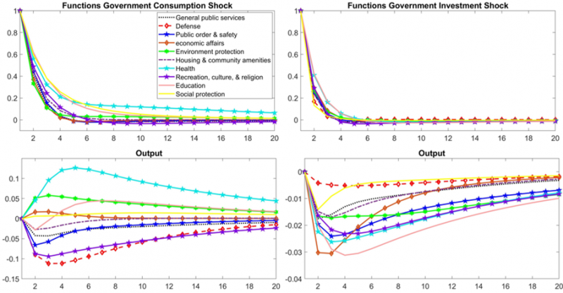
The results from Fig. 3 amplify the heterogeneity of output responses to government consumption and investment shocks. Government consumption spending on functions, such as health and environmental protection6 and education, contributes the most to a positive output multiplier with values of 0.37, 0.31, and 0.14, respectively. Meanwhile, defense, recreation, culture, and religion spending report negative multipliers of −0.69 and −0.54. Moreover, our results show that government investment has a negative multiplier in each reported function.

3. Effects of government spending on sectoral output

In Fig. 4, we take a step back and shed light on the responses of four main sectors subject to government consumption and investment shocks.
We report sectoral output multipliers for agriculture, forestry, and fishing; manufacturing, mining, and construction; wholesale, retail trade, and transportation; and services. Our analysis shows that the response of these four sectors to a government consumption shock is 0.31, 0.16. 0.15 and 0.897. Their response to a government investment shock is −0.29, −0.32, −0.45, and −0.39, respectively. The positive multipliers obtained by the government consumption shock are in line with the results of Bouakez et al. (2023), with distinct differences. First, although both results show a positive output multiplier, our results show a smaller impact, with our results being possibly affected by lower output multipliers in non-US OECD countries. The second difference is that they report values for a disaggregation level of 57 sectors and only for government consumption shock.

4. Effects of sectoral government spending on sectoral output

In Fig. 5, our work takes a middle ground by exploring the sectoral origins of the government spending multiplier in a multi-sector economy. To not complicate the analysis and keep differences at a minimum, and control for other types of heterogeneities, we focus only on sectoral government spending in manufacturing and services and the respective responses in the sectoral output of manufacturing and services.8
Figure 4: Sectoral output responses to a government consumption (LHS) vs. government investment (RHS) shock
 width=
Notes: The figure shows the responses of sectoral output in four sectors as highlighted in colors to a government consumption (LHS) vs. investment shock (RHS). 
Figure 5: Sectoral output responses of sectoral government consumption (LHS) vs. government investment (RHS) shock 
 width=
Notes: The figure shows the responses of sectoral output in two sectors, manufacturing (in blue) and services (in red) as highlighted in colors to a sectoral government consumption in manufacturing and services (LHS) vs. a sectoral government investment (RHS) in manufacturing (in blue) and services (in red). 
Highlighting the results in terms of services and manufacturing becomes important following the work of Cox et al. (2020), that have highlighted the importance of relative price stickiness between sectors for fiscal policy transmission.
A 1% shock in a government consumption shock in manufacturing and services, respectively, produces the max impact response for services at 0.4% while 0% for manufacturing. The multipliers for each are 0.71 and 0. The multipliers in the case of the government investment shock on services and manufacturing display similar differences with −0.20 and 0.

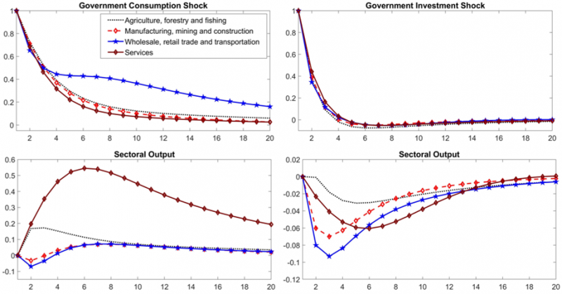
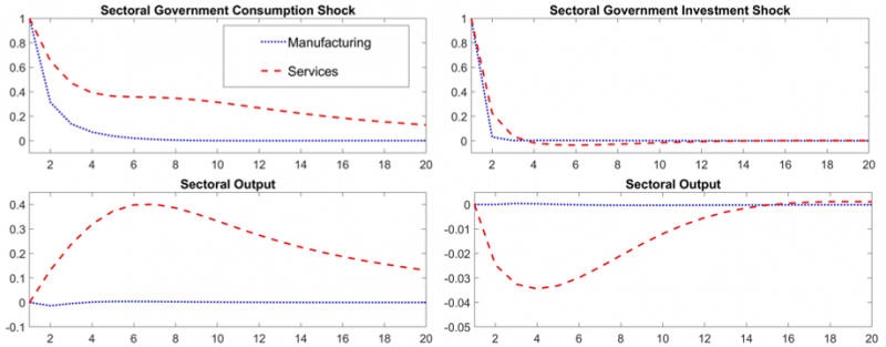
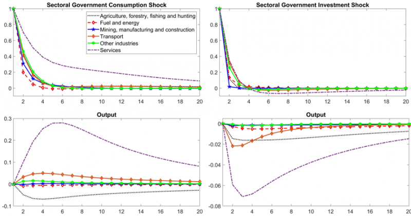
These multipliers are slightly lower than the ones reported for services and manufacturing in Fig. 4, suggesting the possibility of spillovers when looking at the multipliers sectorally to a total government consumption and investment shock. These results are in line with the explanation given by Cox et al. (2020) that reports for the US. The effects of government spending shocks on output are higher in sticky price sectors, such as services, and lower in sectors where firms face more flexible prices, such as manufacturing.9 The results are also in line with Bouakez et al. (2023) since services tend to be more upstream than manufacturing. They do not offer government investment results, which our paper confirms. Our paper contributes to their work by providing evidence for selected OECD countries.

Conclusion

An essential feature of our analysis is relying on separately investigating government consumption and investment, as suggested by Boehm (2020). Our results reveal that government consumption multipliers, either for aggregate output or sectoral output, are, on average, higher than government investment multipliers. For further evidence, we report results relying on the COFOG classification of government activities. By restricting our analysis to only two sectors, we provide an explanation that aligns with Cox et al. (2020) and Bouakez et al. (2023), suggesting variations in price stickiness or sectors’ position in the production network may drive the differences between the sectors.

References

Antolin-Diaz, J., Surico, P., 2022. The Long-Run Effects of Government Spending. Working Paper.
Batini, N., Di Serio, M., Fragetta, M., Melina, G., Waldron, A., 2022. Building back better: How big are green spending multipliers? Ecol. Econom.
Bils, M., Klenow, P.J., 2004. Some evidence on the importance of sticky prices. J. Polit. Econ. 112 (5), 947–985.
Boehm, C.E., 2020. Government consumption and investment: Does the composition of purchases affect the multiplier? J. Monetary Econ. 115 (C), 80–93.
Bouakez, H., Rachedi, O., Santoro, E., 2022. The sectoral origins of the spending multiplier.
Bouakez, H., Rachedi, O., Santoro, E., 2023. The government spending multiplier in a multi-sector economy. Am. Econ. J.: Macroecon. 15 (1), 209–239.
Cox, L., Müller, G., Pastén, E., Schoenle, R., Weber, M., 2020. Big G. Nber Working Papers, National Bureau of Economic Research, Inc.
Gabriel, R.D., Klein, M., Pessoa, A.S., 2023. The effects of government spending in the eurozone. J. Eur. Econom. Assoc..
Hasna, Z., 2022. The Grass Is Actually Greener on the Other Side: Evidence on Green Multipliers from the United States. Working Papers.
Klein, M., Linnemann, L., 2023. The composition of public spending and the inflationary effects of fiscal policy shocks.
Klenow, P.J., Kryvtsov, O., 2008. State-dependent or time-dependent pricing: Does it matter for recent U.S. inflation? Q. J. Econ. 123 (3), 863–904.
Nakamura, E., Steinsson, J., 2008. Five facts about prices: A reevaluation of menu cost models. Q. J. Econ. 123 (4), 1415–1464.
Ramey, V.A., 2020. The macroeconomic consequences of infrastructure investment. In: Economic Analysis and Infrastructure Investment. In: NBER Chapters, National Bureau of Economic Research, Inc, pp. 219–268.
  • 1.

    The dataset includes a yearly balanced panel of 18 OECD countries from 1995-2020. We use government spending data at both the sectoral and functional levels. The OECD COFOG and Stats databases provide most of the data, with the exception of sectoral output, which is obtained from the UN database.

  • 2.

    Following the important results of Boehm (2020) in distinguishing between government consumption and investment and Ramey (2020) which discusses the macroeconomic consequences of infrastructure investment, in all steps of the analysis we clearly distinguish in our results between government consumption and government spending. 

  • 3.

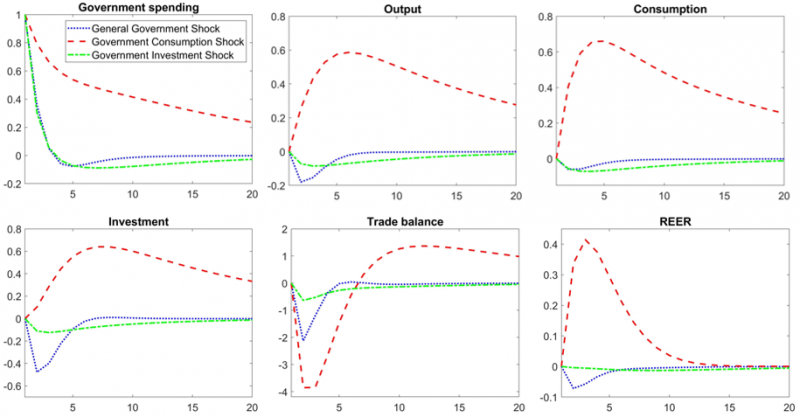
    Total government spending multipliers closely track those of government investment spending in line with the work of Antolin-Diaz and Surico (2022), that argue this finding as suggestive evidence that the long-run effects of government spending on output are significantly shaped by public investment.

  • 4.

    There are no studies that we are aware of that have looked previously at the impact of government investment on the trade balance and exchange rate highlighting an important contribution of this paper.

  • 5.

    The cumulative multiplier shown goes to −0.71.

  • 6.

    The literature on the US economy, such as Hasna (2022) and Batini et al. (2022) for the OECD countries, provide evidence that green public investments tend to produce positive output multipliers. Our paper’s results suggest that not considering government consumption spending on what governments define as the environment could lead to bias in public investment green multipliers. Another explanation could be due to different definitions of what constitutes green and non-green used by the other authors. 

  • 7.

    These results are fairly in line with some of the multipliers reported by Gabriel et al. (2023) on the Eurozone area using sectoral regional data. Nevertheless, they do not distinguish between government investment and government consumption. They report −0.14 for Agriculture after 4 years of impact, 0.69 for services, 0.27 for construction, and 0.66 for the industry.

  • 8.

    The evidence presented in Bils and Klenow (2004), Klenow and Kryvtsov (2008) and Nakamura and Steinsson (2008) suggest that manufacturing can be considered a sector where firms face flexible prices while firms in the services sector adjust prices less frequently.

  • 9.

    They argue that ‘‘when the government demands more goods from all the industries, sectors located upstream raise their production to meet not only the higher demand from the government, but also the additional demand for intermediate goods from their customer industries. The value added of upstream sectors therefore rises more than that of downstream sectors, ceteris paribus’’.

About the authors

Ernil Sabaj

Ernil Sabaj is a Teaching Fellow in Macroeconomics at the Department of Economics, University of Warwick. He has a Ph.D. in economics from the University of Exeter, specializing in macroeconomics and monetary and fiscal policies. Prior to his current role, he was an economist at the Department of Macroeconomics in the Albanian Ministry of Finance and Economy.

Rashid Sbia

Rashid Sbia is a Macro-Fiscal advisor at the Ministry of Finance in the United Arab Emirates and a research associate at Aix-Marseille University, CNRS, EHESS, Centrale Marseille, AMSE, Marseille, France. He holds a Ph.D. in economics from Aix-Marseille University, France, specializing in the oil market, environmental issues, and oil-rich economies. Before moving to UAE, He worked as a senior economist at the Ministry of Finance’s Research Department in the Kingdom of Bahrain. His works appear in prestigious journals, including the Journal of Applied Econometrics, Energy Economics, Energy Policy, and Economic Modeling.

Haytem Troug

Haytem Troug is an economist at the IMF. He has a Ph.D. in economics from the University of Exeter, specializing in macroeconomics. Before joining the IMF, he was a Senior Economist in the Central Bank of Libya. He also worked at UNDP Kuwait as a Consultant and the African Development Bank as a Domestic Economist.

More on these topics

Tags: