Does the shadow economy explain household saving?

We analyze the question of how indicators of shadow economy correspond to the National Accounts values starting with the notion that shadow economy should show up in the difference between household income and consumption in the sense that household (disposable) income is underreported. By contrast, household consumption is more accurate because most of shadow economy income eventually ends up to consumption. Thus, household saving figures should be negatively related to the values of shadow economy: if these values are large, savings should be small, or even negative and vice versa. We test this hypothesis with European cross-country data for 1991-2017 using the so-called MIMIC model calculations as point of reference. Estimation results lend very little support to this hypothesis even though we can otherwise explain pretty well the cross-country variation in household saving and consumption growth rates.

1. Introduction

In the “shadow economy” literature, there are numerous ways of measuring the size of shadow economy. That is no surprise because it is very difficult to measure the shadow economy in the same way as other economic phenomena. Thus, most methods are one way or another indirect, see the extensive survey of e.g. ECE (2008). To sum up very shortly, there are survey studies, studies using the payment media data (e.g. Takala and Viren 2010), employment data, the discrepancies in national accounts, analyses dealing with the tax receipts (tax gap), and different model-based analyses. In the latter category, the most popular set-up is the so-called MIMIC model approach that is propagated by Friedrich Schneider in particular (see e.g. Medina and Schneider (2019)). In this model the unobservable (latent) shadow economy variable is modelled by observable forcing variables using the model restrictions of the (presumed) theoretical model (for details see Schneider and Buehn (2016)).

We use the concept “shadow economy” as an aggregate for all economic activities which are missing from the National Accounts. Thus, they include both so-called grey economy (mainly meaning tax evasion), illegal economy and unreported income. Following the National Accounts, we do not consider household production as a part of shadow economy. As for the shadow economy, estimates of Medina and Schneider (2019) are by far the most widely published and referred values and they cover practically all countries in the world. Our idea is to see how these values coexist with the official National Accounts measures. The hypothesis is that if these estimates are “correct”, shadow economy should show up disproportionally in different National Accounts measures. We have good reasons to believe that shadow economy distorts income measures more than the aggregate demand components. This possibility of measuring the scope of shadow economy is mentioned in almost all literature surveys (e.g. ECE 2008) but thus far there have been very little serious effort to examine whether the idea can be applied with actual data.

Proper analysis cannot be done with the Gross National Product (GDP). That is because of various measurement issues and because the discrepancies are often considered as indication of low quality of statistical compilation. Therefore, we concentrate on just households. In this case, the income and expenditure approaches produce by definition different outcomes and hence statisticians have no incentive to manipulate the discrepancy of these two. Household consumption and income are also surveyed frequently for different statistical purposes (such as income distribution indicators and the consumer price index). Then the basic idea is that household (disposable) income includes a shadow income component that is not included in the National Accounts values of household income. Household consumption may also have a shadow income component, but we have all reasons to believe that this component is much smaller because all income is either consumed or invested. Income from shadow economy is consumed in the same way as other income. In fact, this idea is often utilized in practical anti-corruption and anti-tax-evasion work in the very simple way: individual suspects’ consumption level (housing space, cars and so on) is compared with reported income. Of course, the “true” household consumption includes some items that are not included in National Accounts statistics. Most notably this is true with such “illegal” items as prostitution and drugs but for data reasons we bypass them.

The problem is, of course, that at the level of theory and data we do not have a simple equation consumption = b*income, where the propensity to consume b is universally constant over time and over households/countries. But we may assume for a moment that the relationship between income and consumption would be relatively constant. Then – ceteris paribus – we would expect that in households, and thus in countries, where the shadow economy is large the share b tends to be large or even above one, and the saving rate would be negative. So, we intend to scrutinize whether this is true. Then the question is, do we indeed see that in countries with a large shadow economy the saving rate is small or negative while the opposite is true with economies with small shadow economy. Alternatively, we focus on the dependence of (growth of) consumption on the measures of shadow economy. With consumption growth, we would expect a positive dependence on the size of the shadow economy, given all control variables.

To some extent our approach is related to old study by Pissarides and Weber (1989) where the household (food) consumption income relationship is analyzed from the point of view of grey economy. Pissarides and Weber use the UK Family Expenditure Survey data and end up in estimating an equation where measured income and the indicator of self-employment (plus a set of controls for household characteristics) appear on the right-hand side. Estimation results indicate that substantial amount of underreporting of income is indeed related to self-employment.

2. The data and the model

Starting with shadow economy data. In the Medina & Schneider (2019), there are 158 countries and the data cover the period 1991-2017 for most of the countries. Here we consider the 34 European countries. Most of them are EU countries but we also include Iceland, Norway, Switzerland, UK, Ukraine, Belarus and Russia into the sample.

As for the National accounts data, the key variables are private consumption, household disposable income and the saving rate. We considered both gross and net income Y (and accordingly gross and net saving) but because the measures do not make any noticeable difference in results, we concentrate on the net values. As for the controls, the share of self-employment (emp), the share of agriculture (agr), the per capita income level (gdpc; GDP per capita in constant US dollars), the growth rate of population (Δpop), the growth of real income (Δy), the rate of inflation (π), the real interest rate (rr) and the amount of remittance income; both inflow (rem) and outflow (rex). The latter variables are expressed in US dollars, so they are divided by the respective GDP in US dollars. For scaling purposes, we use the total population numbers. Although the control variables would cover longer periods, we restrict the sample to be the same as in the Medina & Schneider shadow economy sample, i.e. 1991-2017.

The estimating equation for the saving rate is of the following form:

s_it = α_0it + α₁s_it-1 + α₂h_it + α₃Δy_it + α₄π_it + α’X_it + μ_it (1)

where s denotes the saving rate, h the shadow economy measure X the set (vector) of control variables and μ the error term. Subscript i denotes country and t time (year). All variables are expressed in real terms. So, nominal values have been deflated by consumer prices. Thus, e.g. Δy = Δlog(Y/P). At this stage, the basic hypothesis is that α₂ is negative so that an increase in the shadow economy shows up in a larger negative difference between National Accounts’ measures of income and consumption. In a same way we specify the equation for consumption growth as:

Δ_cit = β_0it + β₁Δc_it-1 + β₂h_it + β₃Δy_it + β₄π_it + β’X_it + μ_it (2)

where Δc denotes the growth rate (log difference) of real private consumption growth. With equation (2) the basic hypothesis is that β₂ is positive: an increase in the shadow economy share facilitates higher consumption given the National Accounts’ measure of real disposable income. When we introduce the income growth variable Δy into these two equations we must be aware that there is a difference between the “true” income and the measured income. Suppose that the true income is Y* while the measured income is Y. With consumption, however, the true consumption C* is supposed to equal the National Accounts measure C. The ratio h is assumed to be the share of shadow economy out of measured income. Anyway, h is now (Y* – Y)/Y = Y*/Y – 1, and Δlog(Y*) could approximated as Δh + Δy. Thus, instead of using (the level of) h as the right-hand side variable, we should use its difference in both equations (for more details, see Oinonen & Viren (2021)).

With the saving rate equation, we have an additional problem because also the saving rate contains a measurement error. The “correct” saving rate would be (Y*- C)/Y* instead of (Y-C)/Y. Moreover, the saving rate is highly persistent so that the AR1 coefficient of the lagged value of the saving rate is close to 0.9. This also shows up in the subsequent empirical results. To make things simple, assume that the left-hand side variable is Δs instead of s (in fact, Deaton (1974) uses Δs the dependent variable). Then the skeleton form of the saving rate equation where (a difference in) the saving rate depends only on real income growth can be written into a form Δ((1+h)Y-C)/(1+h)Y = βΔh + βΔy, where β is the coefficient of Δlog(Y*/P) in the saving rate equation. This in turn can be presented in an approximate form Δs = (β(1+h)-1)Δh + β(1+h)Δy implying that the share of shadow economy has a negative effect on the change of the saving rate at reasonable values of h and β while the National Accounts’ income growth still has a positive effect. So, in fact, equation (1) would then take the form:

Δs_it = α_0it + α₁s_it-1 + α₂Δh_it + α₃₁h_itΔy_it + α₃₂Δy_it + α₄π_it + α’X_it + μ_it (1’)

Now we would expect the sign of a₂ to be negative and the sign of both α₃₁ and α₃₂ to be positive. As for other control variables, we use the rate of inflation and the real interest rate. The rate of inflation can be motivated by the Deaton (1974) saving equation where the inflation rate affects saving due to some sort of mismeasurement effect: when inflation goes up, consumers (sampling individual prices) interpret increases of individual prices as changes of relative prices of respective commodities and decrease the demand of those commodities. When we aggregate over households, we end up with a positive relationship between the saving rate and inflation. Obviously, we would expect the inflation has an inverse effect on consumption growth because (roughly) Δs = Δy – Δc.

3. Empirical results

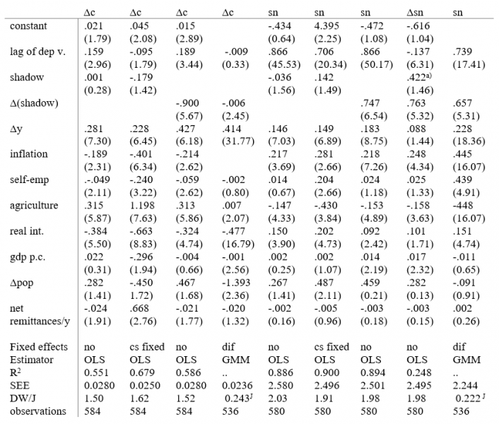
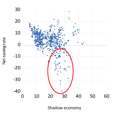
The estimates of equations (1) and (2) are reported in Table 1. Besides OLS we use the (Arellano -Bond) GMM estimator and allow for the possibility that the shadow economy variable is endogenous in the estimating equations (1) and (2). As for the relationship between shadow economy on the one hand and saving and consumption on the other hand, we see from Figure 1 that the saving rate seems to be inversely related to shadow economy. This is, however, very much due to some extreme observations. On one hand we have Romania with very large negative saving rate and very large value for the shadow economy. On the other hand, we have Switzerland with very low value of shadow economy but very high saving rate. But all other observations fail to follow any clear pattern (the case of Romania is discussed in more detail in Rocher et al (2015)).

Results in Table 1 confirm the initial impression that the shadow economy measures do not help predicting neither the level of saving nor the growth rate of consumption. If the level form of the shadow variable is used in the estimating equation, the signs of the coefficients are either “wrong”, or they are not significant at standard levels of significance. Instead, if we use first differences of the shadow economy variable, the t -values are very high, but the signs of the coefficients do not make sense from the point of view of the “shadow economy shows up in income but not in consumption” story. Thus, the estimates imply that an increase in the size of (the change of) the shadow economy decreases consumption growth (given income growth and other controls) and accordingly, an increase in the change of shadow economy increases the National Accounts saving rate. OLS and GMM tell practically the same story.

Table 1. Estimates of consumption and saving rate equations


Numbers inside parentheses are robust t-values. cs fixed denotes fixed country effects. Superscript J denotes the P value of the J-test. Dif indicates that the data are differenced. In the second last column, the dependent variable is differenced. In this column and cell noted by a), the variable is h*Δy according to equation (1’).

Figure 1. Shadow economy share and the net saving rate

Note: Observations in the rounded area come from Greece, Cyprus, Latvia and Romania.

Otherwise we see that both consumption growth and the saving rate are sensitive to the income growth, the real interest rate and the rate of inflation. The saving rate equation works perfectly according to the Deaton’s (1974) “involuntary saving hypothesis” so that inflation does indeed increase saving in the same way as real income growth. The real interest rate does also work in the way consistent to the life-cycle permanent income hypothesis. The coefficients of the self-employment variable are negative in the consumption equation(s) and positive in saving rate equation(s) even if we drop the shadow economy variable from the estimating equations. Clearly, this result is at variance with the idea of Pissarides and Weber (1989) that self-employed persons grossly underreport their income.

4. Concluding remarks

Our analyses show that the most commonly used measure of the shadow economy is not consistent with the idea that shadow economy biases household income more than household consumption. Even though there are several countries where the shadow economy measures correspond to the differences between income and consumption, in most countries they do not. Obviously, this does not mean that National Accounts consumption and income data are equally prone to shadow economy, nor that they are free of the shadow economy bias. Rather it means that the shadow economy measures may be more akin to measurement errors than the National Accounts.

References

Deaton, A. (1977), ‘Involuntary saving Through Unanticipated Inflation’, American Economic Review 67, 899–910.
ECE (2008) The non-observed economy in National Accounts: Survey of National Practices. United Nations Economic Commission for Europe, Geneva. https://unece.org/fileadmin/DAM/stats/publications/NOE2008.pdf
Gyomai, G. and P. van de Ven (2014) The Non-Observed Economy in the System of National Accounts. OECD Statistics Brief 18. http://www.oecd.org/sdd/na/Statistics%20Brief%2018.pdf
Medina, L. and F. Schneider (2019) Shedding Light on the Shadow Economy: A Global Database and the Interaction with the Official One. CESifo Working Paper No. 7981. https://ideas.repec.org/p/ces/ceswps/_7981.html
Oinonen, S. and M. Viren (2021) How does the shadow economy show up in National Accounts? Forthcoming in GUS Economic Review, Issue 2/2021.
Pissarides, C. and G. Weber (1989) An expenditure-based estimate of Britain’s black economy. Journal of Public Economics 39, 17-32.
Rocher, S. and M. Stierle (2015) Household saving rates in the EU: Why do they differ so much? Discussion Paper 005, September 2015. https://ec.europa.eu/info/sites/info/files/dp005_en.pdf
Schneider, F. and A. Buehn (2016) Estimating the Size of the Shadow Economy: Methods, Problems and Open Questions. IZA Discussion Paper 9820.
Takala, K. and M. Viren (2010) Is Cash Used Only in the Shadow Economy? International Economic Journal 24(4), 525-540.
• 1.
The views expressed in this paper are those of the authors and do not necessarily reflect the views of the Bank of Finland or the Eurosystem. The results are based on a forthcoming article in the GUS Statistical Review, Issue 2/2021.
About the authors
Sami Oinonen
Sami Oinonen is an Economist at the Bank of Finland’s Monetary Policy and Research department. His areas of expertise include euro area monetary policy, euro area inflation dynamics, inflation forecasts and international economy.
Matti Viren
Matti Viren is professor of economics (emeritus) at the University of Turku and consultant at the Bank of Finland. Earlier he has served as a research supervisor at the Bank of Finland and as research director at the Government Institute of Economic Research. He has also been the Pre-accession advisor at the Polish Ministry of Finance in 2001-2013. He made his graduate studies at the Universities of Helsinki and Chicago and received his doctorate at University of Helsinki in 1980. Most of his research is related to economic policy and applied macroeconomic analysis.
More on these topics