Forecasting Dutch inflation using machine learning methods

Abstract
This paper examines the performance of machine learning models in forecasting Dutch inflation over the period 2010 to 2023, leveraging a large dataset and a range of machine learning techniques. The findings indicate that certain machine learning models outperform simple benchmarks, particularly in forecasting core inflation and services inflation. However, these models face challenges in consistently outperforming the primary inflation forecast of De Nederlandsche Bank for headline inflation, though they show promise in improving the forecast for non-energy industrial goods inflation. Overall, Ridge regression has the best forecasting performance in our study.

Understanding inflation dynamics is crucial for economic policy and forecasting accuracy. Over the past decades, Dutch inflation has experienced periods of stability and volatility, influenced by major economic events such as the introduction of the euro, the 2008 financial crisis, and the COVID-19 pandemic. While inflation remained relatively stable between 1990 and 2020, the pandemic, subsequent supply chain disruptions, and the surge in energy prices led to a sharp increase, peaking above 10% in 2022.

In this study (Berben et al., 2025), we evaluate the effectiveness of machine learning (ML) models in forecasting HICP inflation and its sub-components in the Netherlands under different economic conditions. While inflation forecasting has been widely explored for large economies, research on smaller nations like the Netherlands remains limited. By benchmarking ML models against a simple time-series model and De Nederlandsche Bank’s (DNB) official inflation projections, we provide new insights into their predictive power before, during, and after the COVID-19 pandemic.

The dataset consists of monthly observations of 129 Dutch and international macroeconomic time-series, covering the period from January 1990 to January 2024. We look at four different target measures of inflation: headline, core, services, and non-energy industrial goods inflation. The explanatory variables can be divided into eleven groups, following McCracken and Ng (2016) and Medeiros et al. (2021): (1) output & income, (2) labor market, (3) consumption, (4) orders & inventories,(5) money & credit, (6) interest & exchange rates, (7) commodity prices, (8) producer prices (PPI’s), (9) domestic prices, (10) price expectations, and (11) stock market.

We examine four distinct ML classes: shrinkage, tree, ensemble, and factor models. Shrinkage models help prevent overfitting by reducing the impact of certain features in a dataset, thereby improving generalization. Tree models employ a tree-like structure to make decisions by splitting data based on conditions. Ensemble models combine multiple smaller models (such as linear regression models) leveraging their collective strength. Lastly, factor models extract key trends from large datasets, simplifying complex relationships.

Furthermore, we examine which model specifications contribute most to improved forecasting performance. We focus on three key aspects. First, we analyze the transformation of the target variable by comparing the effectiveness of path average forecasts, as popularized by Goulet Coulombe et al. (2022) and direct forecasts. Direct forecasts predict a specific month in the future, while path average forecasts generate a sequence of short-term predictions and average them over time, potentially enhancing stability and accuracy. Second, we assess the impact of including or excluding factors in the predictor set. Third, we evaluate whether using the full set of predictors or selecting only targeted predictors leads to better forecasting performance.

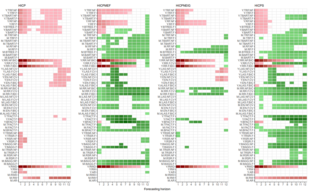
Figure 1 shows on the y-axis the root mean square forecast error (RMSFE) of the ML models relative to the RMSFE of a random walk with drift (the benchmark model), and on the x-as the forecasting horizons, ranging from one to twelve months ahead. A green cell indicates the relative gain in forecasting accuracy of the ML model is at least 5%, red cells indicate there is at least a 5% decline in forecasting accuracy from using the ML model. The colors range from light green(red) to dark green(red), corresponding to a gain(loss) in forecasting accuracy ranging from 5% to 50% or more.

ML model names are abbreviated according to the following convention: [method].[model].[factor].[modelsel]. Method indicates the forecasting approach. “Y” (year-on-year) represents direct forecasts, while “M” signifies path average forecasts, which are derived from month-on-month changes in the price index. Factor indicates whether factors are included in the set of predictors (F), or not (NF). For some models, tuning of the parameters is done in multiple ways. In those cases, [modelsel] can take on the values Bayesian information criterion (BIC) and cross validation (CV).

The first observation is that, in the full sample, none of the ML models consistently outperforms the benchmark forecast for headline inflation. A possible explanation is that, since the volatility of HICP inflation is largely due to volatility in the energy and food components, our set of predictors is not sufficiently rich in terms of energy and food prices related series.

However, ML models significantly outperform the benchmark for core inflation, non-energy industrial goods (NEIG) inflation, and services inflation across most forecasting horizons. This is particularly notable for Ridge regression with path averaging. In addition, tree-based models do not systematically outperform linear shrinkage or factor models and show inconsistent result, indicating that non-linearity is not a common feature of inflation in the Netherlands. Only one tree-based model (M.RF.F) consistently beats the benchmark.

Path average forecasts are more effective than direct forecasts, while incorporating statistical factors or targeting predictors provides minimal additional value.

Figure 1. Heatmap relative RMSFE, full sample (2010M1-2023M12)

Additionally, we assessed the performance of ML models against DNB’s official inflation forecasts (NIPE). DNB contributes to the Eurosystem projection exercises four times a year. These forecasts are based on a suite-of-models approach, and also incorporate expert judgement and announced government policy measures.

When comparing the forecasts of ML models to NIPE, results show that no ML model consistently outperforms NIPE’s headline forecast. This is especially evident for short-term predictions. The performance is also worse for core and services inflation. This could be explained by NIPE’s ability to incorporate tax and policy changes, which the ML models do not account for. However, for NEIG inflation, there are forecasting gains, especially for Ridge regression.

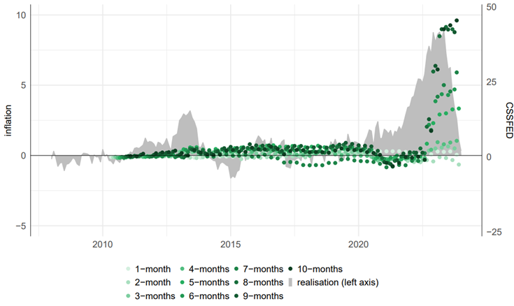
Figure 2 shows the cumulated sum of squared forecast errors difference (CSSFED) for different forecasting horizons for one Ridge regression model. A CSSFED above zero indicates that the forecasts of the ML model has a lower CSSFE up until that point in time, and is therefore more accurate than NIPE. Between 2010 and 2019, the Ridge regression shows marginal forecasting gains over the NIPE forecast for most horizons. However, as NEIG inflation surged from 2020 onwards, the Ridge regression clearly outperformed the NIPE forecasts. This becomes increasingly evident over longer forecast horizons.

To get a better understanding of the key predictors that improved the performance of the Ridge regression in forecasting NEIG inflation, we looked at the contributions of predictor sets since the start of the pandemic. Initially, real activity indicators, expectations, and financial predictors played a major role. However, from late 2021 onward, PPI’s and domestic price pressures, including headline HICP inflation and its components, became the primary drivers. This shift reflects the effects of rising energy costs, supply chain disruptions, and economic overheating.

These findings suggest that some ML models can outperform simple benchmarks, particularly for core and services inflation. However, the forecast accuracy of ML models is often worse than that of DNB’s official inflation forecast. But there are exceptions. Some ML model, particularly Ridge regressions, generate forecasts for non-energy industrial goods inflation that are superior to DNB’s forecast.

Figure 2. NEIG inflation: CSSFED Ridge Regression versus NIPE benchmark