Forecasting with machine learning Shadow-Rate VARs

Interest rates are a core aspect of macroeconomic modelling. Recent literature delves into the complexities of incorporating the effective lower bound into Vector Autoregressions (VARs). This paper focuses on Shadow Rate VARs (SR-VARs). SR-VARs treat interest rates as a latent variable near their effective lower bound (ELB), estimating its unobserved shadow values. The paper studies 16 different SR-VARs with and without stochastic volatility and steady states through the lens of 21 quarterly macro and financial variables from the US. Structural analysis and a real time model evaluation exercise are conducted. We find that the addition of the shadow rate prior improves the forecasting performance of both the macro and financial variables. Structural analysis reveals the differential impact of shocks between models with and without the shadow rate, and underscores the challenges that a central bank faces when the economy is at the zero lower bound.

Shadow-Rate VARs

A pivotal aspect of forecasting is the treatment of interest rates in the modelling process. During recessions, we observe that interest rates can stabilize at their effective lower bound (ELB) for many quarters. This holds true for the Federal Open Market Committee (FOMC) that sets its federal funds rate to not fall below the 0- 25 basis points range. The committee maintained its target range during the Great Recession from December 2008 through December 2015, and this happened again from mid-2020 through mid-March 2022, in response to the recession that was a result of the COVID-19 pandemic. In terms of other economies in the world, the European Central Bank had stabilized its deposit rate to -50 bps. Several central banks in the world are pursuing what is called negative interest rate policies (NIRP) – yet still close to zero. Consistent with the existence of an ELB, policy rates observed under NIRP appear so far constrained to not fall much below zero, see, for example, estimates obtained for the Euro area by Wu and Xia (2020).

This paper is building on the work of Johannsen and Mertens (2021) and Carriero, Clark, Marcellino, and Mertens (CCMM, 2021), who have generalized the unobserved components of the former paper into the VAR setting. This paper uses the block hybrid shadow rate VAR, which allows for the model to capture a stylized fact regarding nominal interest rates: we assume that agents are only affected by the actual interest rates and not the shadow rates for their decisions, yet financial markets (which are represented by the yield curve in our model) are estimated based on the shadow rate values. The forecasting process follows the estimation, as interest rates are forecasted with the shadow rates, while macro variables are forecasted using the nominal interest rates. The CCMM paper argues that models with short and longer term rates tend to forecast better. This could be partially attributed to the different dynamics that are captured by the various interest rate maturities, such as the inversion of the yield curve (a leading indicator for recessions in the US) which is defined as the period where longer term maturities have lower interest rates than the short term ones. Therefore, we are selecting a mixture of short and long term interest rates in a similar fashion to CCMM . While not foolproof, an inverted yield curve has been a reliable predictor of recessions. Historically, most U.S. recessions were preceded by yield curve inversions. Therefore, we use the spread of the 10-year bond with the 1-year bond as the market inflation expectations.

Variable selection, steady states & stochastic volatility

Variable selection is crucial. Macro models can contain hundreds or even thousands of variables (fat data, many predictors). The inclusion of unimportant predictors adds noise to the model, consequently hurting its forecast accuracy. Shrinkage in Bayesian VARs might be optional for small models, but it is pivotal in higher dimensions, as noted by Koop (2013) who showed that large VARs with 20 variables outperform specifications with hundreds of variables.

The LASSO (Tibshirani 1996) is a popular frequentist method for variable selection that penalizes unimportant predictors. Assuming independent Laplace prior distributions for the coefficients of the equations in the VAR model, we get the Bayesian LASSO (Casella and Park 2008). The SSVS prior, developed by George et al. (2008), is a popular algorithm in Bayesian econometrics that chooses whether or not a variable should be included in the model in an automatic fashion based on a test statistic. Finally we also employ the Dirichlet-Laplace (DL) prior developed by Bhattacharya et al. (2015), a hierarchical global shrinkage prior which theoretically induces the optimal shrinkage to the model.

The philosophy of Bayesian econometrics is that more information is good, and we should utilize it in our modelling. Usually, the statistician has priors about the long-run path of variables that could improve forecasting performance. These can be reflected in steady-state assumptions. For example, central banks perform inflation targeting. Villani (2009) develops a VAR steady-state prior and shows improvements in forecastability. Louzis (2019) combined variations of the SSVS prior while also incorporating the steady-state assumptions from Villani. Furthermore, he introduced the estimation of the steady state as a latent variable using the Kalman filter. In this paper, instead of estimating the steady state as in Louzis, we are using long-run forecasts from the Survey of Professional Forecasters. This allows for the steady-state assumptions to differ in each vintage.

There is a vast literature that uses stochastic volatility in BVAR modelling, as it has been shown to improve forecasting performance in VARs. Cogley and Sargent (2005), Primeceri (2005), and D’Agostino et al. (2013), have highlighted the importance of adding time variation to the error covariance matrix of the VAR. This paper explores both homoscedastic as well as stochastic volatility Shadow-Rate VARs.

Forecast performance

One of the most important results of this paper: the infusion of the shadow rate VAR with steady state assumptions results in superior forecasting performance, especially in the longer term horizon. We highlight the importance and usefulness of assessing the forecast performance of the models with both point forecasts and density forecasts. Furthermore we need to assess the model performance during the ELB and outside the ELB, both jointly and separately. The results suggest that all specifications of the shadow rate VAR offer improvements in predicting the fed funds rate in the one step ahead horizon. During periods when the Federal Reserve places its interest rate near the zero lower bound, point forecasts of the SR-VAR models improve both the fed funds rate forecasts and the yield curve forecasts. Furthermore, the shadow rate specifications retain their importance in forecasting core macroeconomic variables even in periods outside of the ELB.

Shadow rate estimates

This section compares machine learning shadow rate models against the Wu-Xia benchmark during two periods: real-time estimates from 2009q1 to 2015q4, and full sample estimates up to 2019q3.

The figure below visualizes a key finding of this paper, which is the high correlation (0.81) that the SSVS SR-VAR with stochastic volatility model exhibits with the Wu-Xia shadow rate in its real-time estimates. However, this correlation drops to 0.09 during the full sample period. Despite the close real-time correlation with the Wu-Xia rate, end-of-sample estimates show little correlation.

Figure 1: Full VAR – Shadow rate estimates for model:
Stochastic Search variable Selection-Stochastic Volatility-Shadow Rate
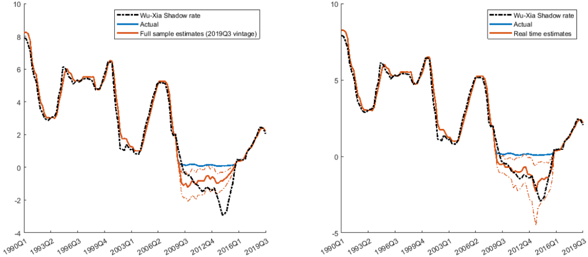Notes: Full sample (left) vs real time (right) shadow rate estimates for the SSVS-SV-SR model. The blue line shows the actual fed funds rate, the black dashed line is the Wu-Xia Shadow rate estimates, the thick red line represents the median and the thin red line are the [10,90] quantiles of the shadow rate estimates.

The shadow rate Minnesota models, both with and without steady states, show high correlation with the benchmark in the full sample. However, their real-time estimates show little correlation with the Wu-Xia rate. This suggests these models may better capture shadow rate dynamics with the revised macroeconomic data available in 2019q3. The following table summarizes those findings by presenting the correlations of the shadow rate models and their summary statistics.

Table 1: Machine learning shadow rates vs the Wu-Xia benchmark
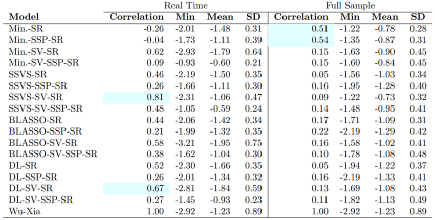Notes: Statistical analysis of the shadow rate estimates. The correlation coeefficient column presents values of the correlation between the real time and end of the sample shadow rate estimates, against the Wu-Xia shadow rate. The reference sample is 2009q1—2015q4 for the real time estimates, and the vintage of the end-of-sample estimate is 2019q3.

The standard deviations across models vary, with the BLASSO-SV-SR model showing the highest, indicating greater volatility in its shadow rate estimates. However, all models produced in this study have consistently smaller dispersion from the mean.

Shadow rate VARs and the Price Puzzle

When the federal funds rate gets hiked or when any central bank increases its policy rates, this is to tame an inflationary cycle in the economy. Or at least that is the expectation. Balke and Emery (1994) describe the bond market’s reaction in early 1994, where a 25bps increase of the fed funds rate resulted in an increase of longer term bonds in the next month, or in other words – markets started discounting an upcoming inflationary increase. Impulse responses of VARs produce the same result as in the above example, thus showing a positive relationship between prices and the policy rate, a result which goes against theory. This came to be known as the price puzzle, as described by Sims (1986, 1992) and many others.

In this paper we perform structural analysis on our models, without any identification assumptions. We include the Producer Price Index for all commodities as Sims suggests and also include a measure of inflation expectations. We are following Koop et al. 1996 using the Generalized impulse response functions. This setup nullifies the impact that the ordering of the variables has when we construct our structural VAR. Our results show that the PPI measurement of inflation is consistent with theory in the long run and does not fall into the price puzzle category. Furthermore we see that the IRFs differ in magnitude from vintage to vintage.

The impulse responses (from now on IRFs) shown in the next figure compare two vintages: one that is during an ELB episode (2012 Q1) and one that is not (2017 Q1) and two models. The IRFs of the shadow rate SSVS with steady states and stochastic volatility show that an upward shock in interest rates will result in an increase of unemployment, and a contraction of consumption, employment, cash flow, housing starts and the industrial production. Inflation expectations fall while prices, measured by the Producer Price Index (PPI), lag by five quarters for both the 2012 Q1 vintage and the 2017 Q1 vintages before the cumulative effect goes to negative territory.

Figure 2: Shadow rate vs non-shadow rate
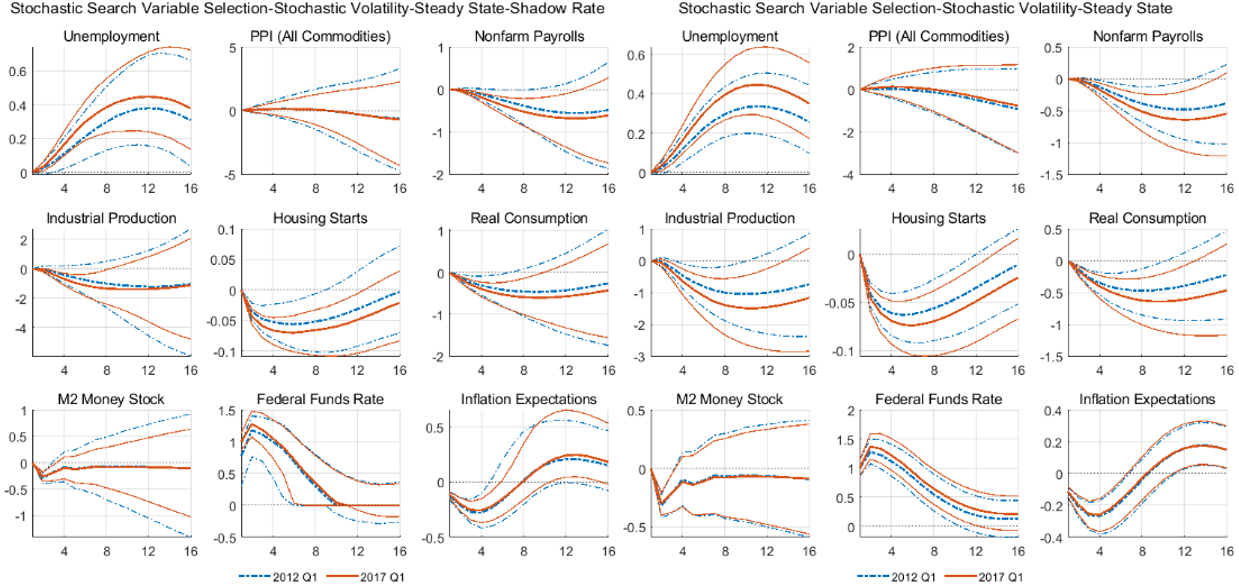Notes: Generalized impulse responses of two large 21-variable VARs. The graphs show the IRFs for a positive standard deviation shock to the Federal funds rate. The 2012 Q1 and 2017 Q1 vintages are represented by the dashed blue lines and the solid red lines respectively. Horizon of 16 quarters, posterior means and 68% credible sets.

The next figure shows the IRFs produced by a negative shock to interest rates, where the central bank tries to enact expansionary monetary policy while interest rates are at the ELB in the 2012q1 vintage. We observe that all variables in the model, are impacted less by a negative shock on interest rates when we are at the effective lower bound. The IRFs of the shadow rate model capture the fact that there is limited leeway for expansionary policy – only half of the shock is produced compared to the model without shadow rates in 2012q1.

Figure 3: Expansionary monetary policy shocks in Shadow rate VARs
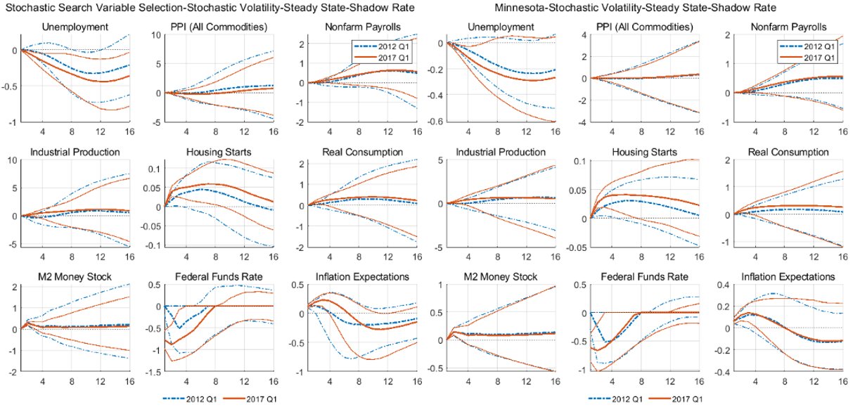Notes: Generalized impulse responses of two large 21-variable VARs. The graphs show the IRFs for a positive standard deviation shock to the Federal funds rate. The 2012 Q1 and 2017 Q1 vintages are represented by the dashed blue lines and the solid red lines respectively. Horizon of 16 quarters, posterior means and 68% credible sets.

Our empirical exercise reveals that the impact of monetary policy varies significantly at the ELB as the central bank’s capacity to stimulate the economy is limited. This results in a subdued expansionary monetary policy shock with muted effect on inflation expectations and consumption. Unemployment falls roughly half of what is observed outside of the ELB.

Concluding remarks

Interest rates play a fundamental role in the transmission of monetary policy and are thus crucial in macroeconomic modelling. The existence of the effective lower bound, which is mandated by central banks, creates non-linearities that are rarely taken into account. This is studied by examining shadow rate VARs that assume economic agents are acting based on real interest rates, while the financial markets are taking the shadow rates into account.

The study evaluates the forecast performance of various shadow rate VAR models across different periods and presents findings that the shadow rate models, particularly those with steady-state assumptions and stochastic volatility, enhance forecast accuracy. This is highlighted by consistent gains in fed funds rate and yield curve predictions. The shadow rate models also improve forecast accuracy for various economic indicators across different evaluation windows, with notable improvements in longer-term forecasts and specific gains in density forecasts for unemployment and consumption.

We then benchmark these shadow rate estimates against the Wu-Xia, which is a reference point in the shadow rate literature. We find that a set of the models achieve real-time estimates that are strongly correlated with the Wu-Xia estimate.

The paper also explores the price puzzle in economic theory and proposes solutions through the structural analysis of models without identification assumptions. It finds that the shadow rate VAR produces Producer Price Index measurements of inflation that are consistent with theory in the long run. The impulse responses show that interest rate shocks lead to increased unemployment and reduced economic activity. We find that the addition of the steady-state prior produces impulse responses that are more closely aligned with the theoretical framework of inflation’s reaction after an interest rate shock.