GDP revisions are not cool: the impact of statistical agencies’ trade-off

Official estimates of economic growth are regularly revised and therefore forecasts for GDP growth are done on the basis of ever-changing data. The economic literature has intensively studied the properties of those revisions and their implications for forecasting models. However, much less is known about the reasons for Statistical Agencies (SAs) to revise their estimates beyond the timeliness of their data collection. We show that SAs behave as risk managers who have an implicit interest (loss function) in not revising their initial GDP estimates too much, while they are much more open to revise GDP expenditure components over time. More than a curiosity, we exploit this resulting cross-correlation of revisions among GDP components to build a model to better forecast GDP.

Statistical agencies’ trade-offs

Gross Domestic Product (GDP) is one of the key data series followed by Central Banks to inform monetary policy decisions. GDP is produced by Statistical Agencies (SAs) that assign utmost importance to its accuracy, but they also face several trade-offs which affect data quality. Firstly, there is a well-known trade-off between data timeliness and accuracy. While users of the official statistics expect them to be available as soon as possible to measure the current state of the economy, statisticians are constrained by the availability of data sources. For instance, the flash estimate for the euro area GDP is available as soon as 30 days after the quarter-end but it is based on incomplete information as the more accurate data arrives later from structural annual sources. Secondly, when the first full GDP breakdown is released, it is compiled using different approaches: production-, income-, and expenditure-based. On the production side, GDP measures the sum of the gross value added created through the production of goods and services in the individual sectors of the economy. On the income side, it measures the sum of all incomes generated by the production of goods and services. Finally, on the expenditure side it measures the sum of domestic and (net) external demand for the produced goods and services (i.e. private and government consumption, investment, net trade, and inventories). To ensure a consistency between the GDP expenditure components and the GDP total figures, SAs need to make maximum use of available sources and to optimise the revisions.

As a result, GDP and other National Accounts statistics are regularly revised, which means that macroeconomic forecasts are based on ever-changing information. In our paper we show that taking into account the trade-offs faced by SAs, in particular the bottom-up derivation approach based on expenditure components, and combining it with data revision analysis to study patterns and cross-correlations among GDP components can be helpful for forecasting aggregate GDP.

GDP revisions literature

Users of data understand the uncertainty surrounding the early GDP announcements. Following the seminal paper of Mankiw (1984), several papers in the literature have shed light on the properties of GDP revisions and how those revisions affect forecasting. Among them, Mankiw (1986), Mork (1987), Croushore and Stark (2003), Faust et al. (2005), Arouba (2008), Clements and Galvao (2010) and many others. For an extensive survey on the impact of data revisions in many different contexts, see Croushore (2011).

The basic idea of those papers was to check if revisions to GDP were fulfilling desirable statistical properties (rationality tests), i.e. revisions should not be biased and therefore present a zero mean, revisions should be small compared to the volatility of the GDP series itself, and finally they should be unpredictable, which means that they carry information (news). Otherwise, if they are predictable, then they would be considered as noise and therefore no need to be used for a forecasting exercise. Many of the above cited studies conclude that GDP data revisions are predictable and therefore noise questioning their usefulness in forecasting models. There should be enough information in the first announcement. Against this idea, another strand in the literature has nevertheless shown the usefulness of using vintages for forecasting, see for example Garrat et al. (2008), Kishor and Koenig (2012), Clements and Galvao (2012; 2013), and Carriero et al (2015). These papers mainly incorporate GDP vintages and its revisions at a vector autoregressive (VAR) approach.

In our paper we first investigate the properties of data revisions, including news vs noise analysis, and we seek for the reasons regarding the limited change in the GDP initial data announcements. After documenting properties and patterns observed among the revisions to GDP and its expenditure items, we then construct a components-vintage VAR (CV-VAR) model that outperforms (in terms of Root Mean Squared Forecast Errors (RMSFEs)) a standard vintage VAR for forecasting initial GDP announcements.

Are revisions to the GDP growth rate statistically 0?

We postulate that SAs consider the initial GDP growth estimates to be accurate enough and they internalise the trade-off between publication timeliness and reliability as minimising GDP revisions. It means that revisions to the GDP growth rate should be statistically 0. We test this hypothesis by showing that revisions to some expenditure items in National Accounts statistics regularly compensate each other.

We use a dataset that contains vintages of real GDP and expenditure components for Germany, France, Italy, and Spain. The data sample covers period 2002-2023. However, given the specificity of statistical data collection during the 2020-22 pandemic which had an impact on data revisions, we split the sample into pre- and post-COVID periods. Data are those published by Eurostat as part of National Accounts.

The analysis of the data revisions shows that indeed new incoming information does not significantly change the initial GDP estimates, but it changes other GDP sub-components on the expenditure side which then cancel each other out at an aggregate level.

Cross-correlation among revisions to expenditure components

We further show that some of the revisions to expenditure components exhibit high correlation with each other.

Figure 1: Correlation coefficients among revisions to GDP sub-components

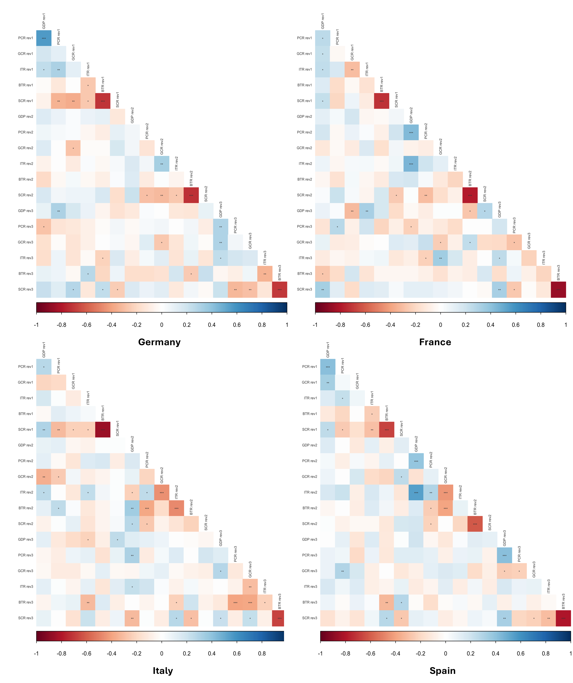
Notes: correlation coefficients among 1st, 2nd, and 3rd revisions to GDP sub-components (PCR-private consumption, GCR-government consumption, ITR-investment, BTR-net trade, SCR-inventories). We show the statistical significance with asterisks, ***: p<0.01,**:p<0.05,*:p<0.1.

Looking at Figure 1, there is a strong indication of the phenomenon we have in mind. For all countries and all vintages, the revision of the contribution of inventories has a significant negative correlation with the revision in the trade contribution. Moreover, using simple econometric analysis we find that the revision of the contribution from the external sector explains about 50% of the change in inventories across countries and vintages.

Components vintage VAR (CV-VAR)

Incorporating these results into a components vintage VAR (CV-VAR) model, we find that a dis-aggregated forecast of initial GDP announcements using the expenditures components contribution revisions performs better in the short-run than the standard vintage VAR (V-VAR) model using the aggregate revisions. We find that the CV-VAR approach can improve the forecast of the initial announcements for most of the cases compared to the standard V-VAR model that does not utilise the expenditure components. In particular, the one period (h=1) ahead forecasts generate lower average RMSFEs across all the countries, and sub-periods, in our sample apart from Italy, compared to the standard V-VAR model. In some instances, these improvements are also statistically significant and there is no case where the V-VAR model generates a statistically significant better forecast than our CV-VAR model for the initial GDP announcement. When it comes to the four periods (h=4) ahead forecasts we find that the two models are not very different but still there is no evidence that the standard V-VAR approach can outperform our CV-VAR model. We even find that for Spain during the pre-COVID period our CV-VAR model produces statistically significant better forecasts for GDP’s initial announcements over the standard V-VAR approach.

Table 1: Forecast comparison of GDP initial announcements 1 and 4 periods ahead

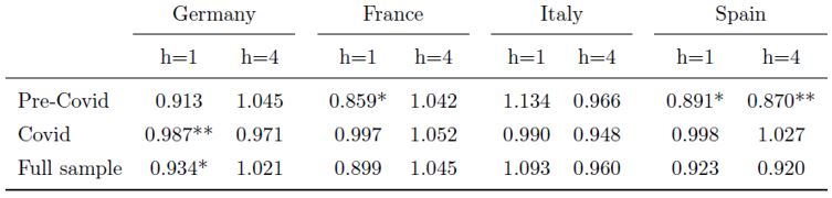
Notes: The results above show the ratio of the average RMSFEs when comparing the forecasts between the standard V-VAR model without the components and our real-time CV-VAR model with components. A value less than one indicates that the CV-VAR approach performs better on average than the alternative. The Diebold-Mariano statistic is also applied and we show the statistical significance with asterisks, ***: p<0.01, **: p<0.05, *: p<0.1.

These results show significant evidence that the use of the revisions of the expenditure component contributions instead of the aggregate GDP revisions can improve the forecasts of GDP initial announcements in the short run.