Abstract
Gold is widely recognized for its role in managing portfolio risk, but its long-term return profile is not as well understood. Existing research often mischaracterizes gold, relying on narrow perspectives or data that fail to capture its true nature. This paper by the World Gold Council introduces the Gold Long-Term Expected Return (GLTER) model, a robust framework that reflects gold’s unique position as both a real good and a financial asset. By linking gold’s price behaviour to economic growth and financial market factors, the model explains why gold has consistently outpaced inflation over the past 50 years. More importantly, it offers a structured approach to estimating its future returns—one that aligns with capital market assumptions for other asset classes.
While gold’s contribution to managing portfolio risk is well established, supported by a large body of work devoted to its hedging characteristics, its contribution to portfolio return is not. Frameworks for estimating gold’s long-term returns exist but fall short of a robust approach that aligns with the capital market assumptions for other asset classes. This paper sets out such a framework, accounting for gold’s unique dual nature as a real good and a financial asset.
Publications tackling gold’s expected return have generally concluded that gold’s primary function is as a store of value, implying a long-run co-movement of gold with the general price level (CPI). Alternative approaches using risk premia estimations or bond-like structures with embedded options produce similar results.
And while existing research is rich in insight, two features frequently pop up that, in our view, mischaracterise gold and have led to biased conclusions:
In most cases, existing research lands on an expected long-run real return ranging between 0% and 1%.
We instead show that gold’s long-run return has been well above inflation for over 50 years, more closely mirroring global gross domestic product (GDP), a proxy for the economic expansion driver used in our other gold pricing models.
Our simple yet robust approach – which we refer to as Gold Long-Term Expected Return or GLTER – uses the distribution of above-ground gold stocks analysed via different demand categories as a foundation and starting point.
The drivers of gold buyers across various demand segments – jewellery and technology fabrication, central banks, financial investment, retail bars and coins – are crucially broader and more important than existing theories suggest. In addition, although financial market investors tend to dictate price formation in the short term, they are less dominant in the long term.
We show that the gold price over long horizons is mainly driven by an economic component, proxied by global nominal GDP, coupled with a financial component, proxied by the capitalisation of global stock and bond markets, that balances the overall relationship. Third-party inputs are then used to estimate long-term expected returns for gold.
Gold’s dual nature, as both a real good and a financial asset, means that its value is not easily explained by traditional asset pricing models. This is further complicated by gold’s continued use as a monetary asset within central bank reserves, despite the ending of the Gold Standard and the mandatory requirement to hold gold as reserves more than five decades ago.
As gold does not generate any cash flows, traditional discounted cash flow models are not applicable. Generally, commodity pricing models also fall short given gold’s unique and ever-growing above-ground stock that, among other things, diminishes primary production as marginal supply. Unlike most other commodities such as oil and wheat, gold cannot be consumed in the sense that its consumption makes it disappear.
Several theories suggest that gold’s expected return should equal the inflation rate. These include the work of Hotelling. His work on exhaustible resources proposes that commodity prices are linked to interest rates, implying an opportunity cost of production. Since interest rates and inflation rates co-move over longer horizons, price changes in commodities and the cost of production both move with interest rates (as proposed by Hotelling) and inflation rates.
But focusing on inflation, interest rates or mining costs as the main driver of gold prices is too narrow for several reasons.
First, gold has significantly outperformed both inflation and the risk-free interest rate: its average annual compounded return (in US dollars) from 1971 to 2023 was 8% for gold vs 4% for US CPI and 4.4% for the US 3-month Treasury.#f1 The probability that such excess returns are due to chance, rather than a characteristic of gold, is very low.
These returns also reject claims that the zero or low correlation of gold with the market, measured as a zero beta with respect to the market in a capital asset pricing model framework, implies that the return of gold is equal to the risk-free rate.2 Gold returns are not a proxy for the risk-free rate theoretically and indeed are greater empirically.3
Second, some research suggests producers are marginal price setters by linking gold prices to mining costs.4 However, it has been shown that miners react to higher gold prices by mining more costly deposits – driving mining costs up, and vice versa.5 Thus, causality appears to work in the opposite direction to that suggested by such research.
Finally, the large above-ground stock of gold comprises an ever-growing source of supply ready to return to market, competing with primary production that contributes less than 2% to the stock each year. This makes the gold price not only less sensitive to production but also materially distinguishes gold from other commodities.
The bulk of existing research places financial investment at the forefront of price determination for gold but while the short-term impact of financial markets is undeniable, the long-term importance of other sources of buying is even more so.
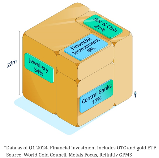
The estimated above-ground stock of gold, at 212,582 tonnes, which we depict as a cube, is a balance sheet snapshot of gold ownership (Figure 1). It is remarkable for a number of reasons.
The cube illustrates how the total stock of this ubiquitous metal could occupy a physical space barely larger than three Olympic-sized swimming pools. In addition, it reveals how little financial investment – (referring here to physically backed gold ETFs and over-the-counter (OTC) physical holdings) has been amassed by market participants over the years in relation to other sources of demand – a misleading statistic given the vast volumes of gold that flow through financial centres every day.
That so much of this hypothetical cube is not owned via financial instruments implies that any explanation of its total distribution must consider factors beyond those solely linked to the day-to-day decisions of financial market participants.
The distribution of the cube also suggests that the price of gold has been driven by two distinct components: an economic component combined with a financial component.
Figure 1. The cube of above-ground gold stocks shows gold’s ownership across sectors of demand
Estimated above-ground gold holdings by category*
We illustrate an example of these dynamics in Chart 1 using quarterly data from 2000, adding COMEX futures net positions to the mix to capture derivatives activity.6 This compares the cumulative net consumer flows (jewellery plus technology minus recycling) to flows relating to gold financial instruments (gold ETFs, plus OTC net buying and net long futures positions). The volume from gold accumulated through financial instruments is more than twice as volatile as net consumption, yet accumulates at a much lower rate.
It is this accumulation – whether for individuals, the reserves of select central banks or even investment for long-term savings – that we attribute to an economic component. The financial component represents, more tactical considerations, such as hedging demand, whether from individual or institutional investors.7
Chart 1. Financial investment is more volatile and accumulates more slowly than consumer and retail bar and coin demand
Cumulative gold demand since across categories*
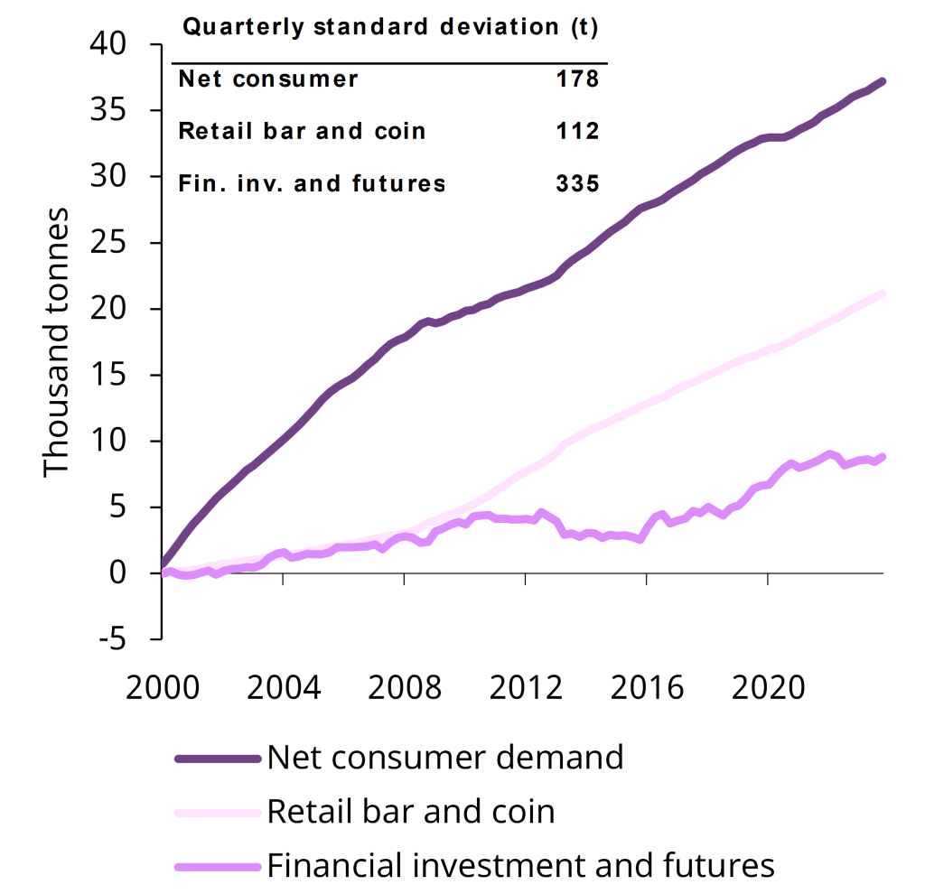
*Data as of Q4 2023. Consumption represents jewellery and technology less recycling. Retail bar and coin follows our standard definition as reflected in Supply and demand notes and definitions. Financial investment and futures captures OTC, ETF and COMEX futures demand. Source: Bloomberg, Metals Focus, Refinitiv GFMS, World Gold Council.
There is a common pitfall in establishing an expected return for gold when using historical data to test a theory empirically. Generally, more history is preferable to less, as more observations increase one’s confidence in the analysis. Capital market assumptions for long-term stock and bond returns commonly use data from 1900 or earlier.8 Replicating this for gold creates one glaring issue: for the best part of the 20th century gold prices were determined by the conversion rate established by central banks and governments. This means that gold was money, linked to the US dollar at a fixed price that was only adjusted sporadically. As such, investors were not always able to use it in practice as an inflation hedge or an equity market hedge. And in the US, citizens were barred from acquiring gold as an investment from 1933 to 1974.
For gold, while its historical performance during Gold Standard periods is an interesting reference, it is truly its market structure and behaviour post-1971 that matters most.
By way of an example, to value a company and assess its expected return, one needs to apply the analysis to the business it will be rather than to the business it has been. If the two are materially different, then past is not prologue. Take Finnish company Nokia, established as a manufacturer of rubber cable and boots until the early 1990s when it morphed into one of the global leaders in the telecoms industry. Applying valuation metrics to Nokia as a boot maker in the early 1990s would have been as fallible as valuing gold in 2024 based on its performance as money during the first half of the 20th century.
We proxy the economic and financial components using real-world economic and financial variables with global nominal GDP as a proxy for the economic component that captures the flow of capital from income to gold.
Our financial component is proxied using the capitalisation of global equity and bond markets – the global portfolio. It captures the capital available for investors to reallocate income and wealth.9
Our regression analysis reveals that GDP is the primary driver of the gold price in the long run.
Table 1 presents two different regression result specifications. Model (1) examines the co-movement of gold prices with only GDP. This model yields a positive and statistically significant relationship. However, the insignificance of the Phillips-Perron unit-root test result suggests that this simple system does not satisfactorily explain long-run gold prices.
Table 1. Gold’s long run behaviour is explained by global GDP and global portfolio capitalisation
Gold long-term price model (1971-2023)
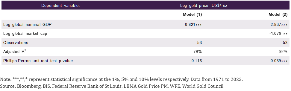
Model (2), which we have labelled Gold Long-Term Expected Return or GLTER, uses both components to create a stable long-run system. A relatively larger coefficient for GDP estimated at 2.8 means that, all else being equal, a 1 unit rise in GDP is associated with a 2.8 unit rise in gold. As we log both sides, these can be interpreted as percentage changes. The negative coefficient for the global portfolio (-1.07) moderates this relationship, as gold is competing for a share of savings, with a one-unit rise in the capitalisation of equity and bond markets associated with a one-unit reduction in gold prices. Once growth as the primary driver of gold prices has been accounted for, we are left with this substitution effect between gold and the global portfolio.
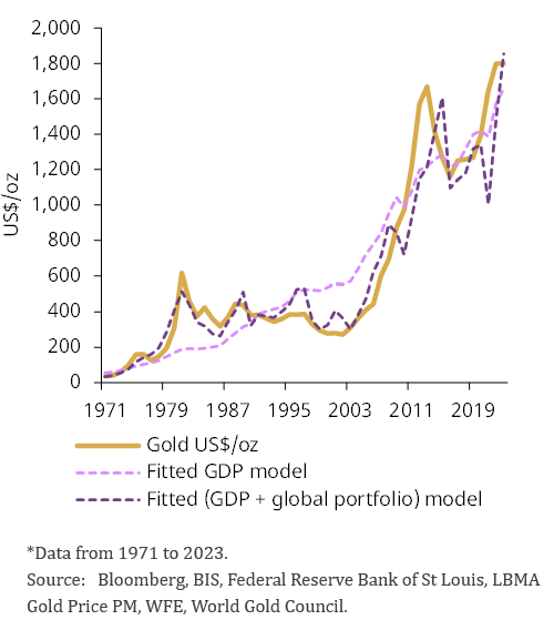
Chart 2 plots the results of these regressions. The purple dashed line shows the modelled gold price using GDP only, with the errors being particularly pronounced in the 1980s and the 2000s. The graph also displays the fitted line of the full model (black dashed) using both global nominal GDP and global portfolio capitalisation. The use of two variables rather than one yields a better fit with the price of gold. While it is not surprising that two variables provide a better fit than one, it is notable that the financial variable significantly reduces the deviations from the long-term relationship.
Crucially, using only an economic component to explain gold prices produces models with rather prolonged periods of disequilibrium. Accounting for gold’s dual nature makes for a much more nuanced explanation of gold’s long-run price path.
Chart 2. Gold is influenced by GDP and the global portfolio in the long run
Actual and modelled gold prices*
We convert our findings into a framework that is perhaps more accessible to investors: the building block approach used widely by practitioners assessing long-term capital market assumptions.
Gold’s price relationship with GDP and the global portfolio can be extended to represent a relationship in return terms. This converts and simplifies these level components into the following relationship:
r g = β1 * GDP Growth – β 2 * global portfolio growth
where rg are annual gold returns, GDP growth is annual global nominal GDP growth and global portfolio growth reflects the growth in market capitalisation of equities and bonds, both in US dollars.
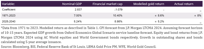
In Table 2 we use the results of Model (2) to predict an 8.6% annual average return for the period 1971–2024, versus an actual return of 8% over that period. Using external forward estimates for GDP growth and the global portfolio, the model predicts an annual average return of 5.2% for the next 15 years.
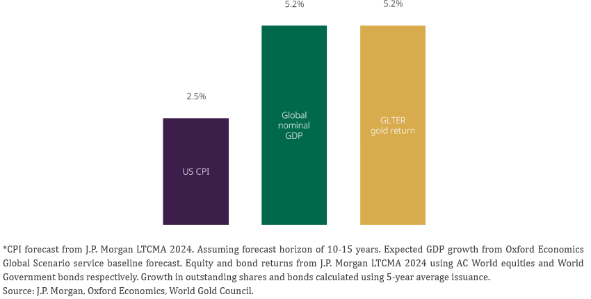
The estimated average gold return over the 2025-2040 period in excess of 5% per year is well above that produced by most other models (Figure 2). Specifically, the estimate exceeds common long-term return assumptions such as a zero real return (2.5% nominal in line with expected CPI inflation) over the next 15 years, 10 or a gold return equivalent to the risk-free rate (2.9% for short-term US Treasury bills).
This is lower than the historical return we’ve observed, largely down to a lower expected growth in global GDP. However, a lower nominal GDP growth rate is likely to impact all asset return, not just gold.
Table 2. Gold’s return will be influenced by future expected growth
Historical and modelled gold annualised returns*
In our view, any model that fails to account for economic growth alongside financial factors will prove insufficient in establishing gold’s long-term expected return. Our novel contribution highlights the theoretical and empirical importance of economic growth and gold’s role in global portfolios in driving gold prices in the long run. GLTER complements our other gold pricing models, GRAM and Qaurum, where economic expansion is present but not a central driver given their short- and medium-term focus. And it explains why gold’s long-term return has been, and will likely remain, well above inflation.11
Figure 2. Gold’s return over the coming decade will be influenced by expected global economic growth
Expected annual growth in US CPI, global nominal GDP and gold price using GLTER model (2025-2040)*
A one-sided T-test of gold’s excess return vs CPI and the risk-free rate gives a p-value of 0.04 and 0.05 respectively. An alternative way to express this is that the probability of observing such a return if the expected excess return is zero, is very low.
Baur and Lucey (2010).
He, O’Connor and Thijssen (2022).
Levin, Abyankhar and Ghosh (1994).
O’Connor, Lucey and Baur (2016).
Although COMEX futures ownership, and indeed that on other futures exchanges, does not explicitly exist in the cube, eligible and registered stocks do, and some positions in the futures market are hedged using physical gold. More importantly, we add futures to the mix as they play an important role in price discovery in the short term and add to short-term turnover in markets.
The dual nature of gold drivers was covered extensively by Goldman Sachs as part of its Fear and Wealth framework; see Appendix D for our analysis. In addition, the model developed by Barsky et al. (2021) employs real GDP as a significant driving factor behind the price.
Global Investment Returns Yearbook 2024 | UBS Global. Long-Term Capital Market Assumptions | J.P. Morgan Asset Management (jpmorgan.com).
As such these variables are a composite of prices and issuance. The marginal negative coefficient for bonds in particular may reflect that issuance must often be absorbed regardless of yield, as we saw in Europe after the Global Financial Crisis, which might crowd out investments in alternatives such as gold.
J.P. Morgan LTCMA 2024.
Using J.P. Morgan long-term capital market assumptions, GLTER suggests that gold return between 2025-2040 is expected to be above that of US Intermediate US Treasury bonds and World government bonds.