How to measure inflation volatility. A Note.

1. Introduction

Inflation and price-level changes are not strictly the same concept. A price-level change is a simple rate of change measurable with only two points in time, including a transitory and a permanent components.1 By contrast, strictly speaking, inflation is a long-term concept only measurable in a steady state situation and cannot include short-term price level movements.2 However, generally speaking, it is common to identify inflation with the price-level change and differentiate between permanent and transitory components. From now on, we will adopt this terminology. The inflation volatility relates to unexpected short-term movements in prices as a result to any shock type, so we propose estimating inflation volatility assuming rational inattention3 in creating uncertainty beliefs on current inflation, such that prices incorporate new information with certain delay. More precisely, we define inflation conditional variance as a weighted average of squared one-period ahead forecasting errors, where the weights follow an exponential decay law that assigns higher weights to recent shocks. Inflation volatility is the annualized squared root of inflation variance. The rate at which news arrive to the market determines the exponential decay intensity, such that a higher rate relates to higher decay intensity. Our approach subsumes other models that have been traditionally used and overcomes these in volatility forecasting exercises.4

2. Inflation volatility

How do we measure inflation volatility? This is an important question with no trivial answer. Inflation volatility intends to estimate inflation’s “average” deviation from its expected value. The first challenge emerges, how do we differentiate between expected and unexpected inflation dynamics? We model the inflation dynamics to identify unexpected price changes or one-step forecasting errors and distinguish between permanent and transitory components of inflation. Next, a second challenge emerges. How do we average historical forecasting errors to estimate inflation volatility? Since volatility is a latent variable, we define a conceptual framework based on the assumption of rational inattention and sticky prices that assumes a decreasing dependence of conditional inflation volatility on past forecasting errors, such that the contribution of today’s innovation to volatility is maximum and decreases exponentially with time. We suggest using the frequency of news arrival in the market to estimate the weighted decay coefficient for shocks. This means that when the news arrival rate is low, the agent tends to give historical shocks a similar weight so that inflation volatility will be equally dependent on past shock sizes. However, when news arrives on the market, the agent will prioritize the information on recent shocks over historical ones to estimate conditional volatility. Our statistical model for inflation volatility can be seen as a restricted GARCH model that weights squared forecast errors exponentially with a decay factor estimated under the assumption of rational inattention.

3. Inflation target. Inflation below or above 2%?

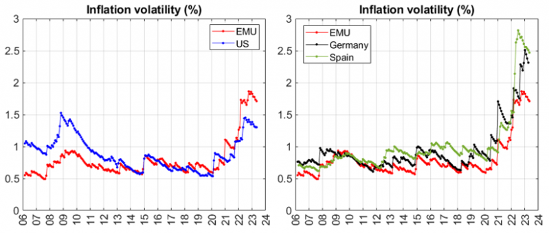
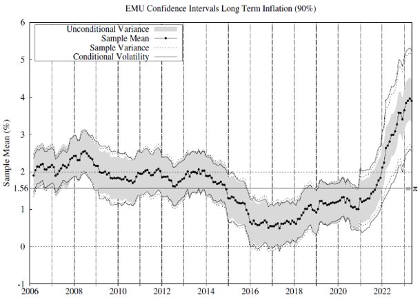
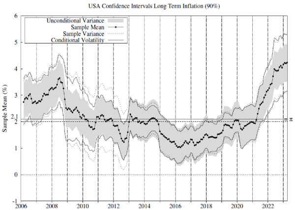
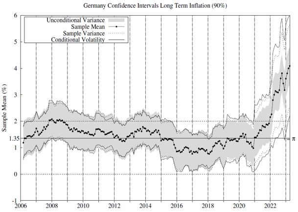
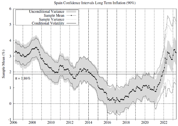
We test whether there is statistical evidence of inflation exceeding 2% in these countries and jurisdictions since 2006. To this end, we estimate the conditional inflation permanent component per each jurisdiction and country as the moving average inflation and use the conditional volatility series in Figure 1 to implement the statistical tests. Figure 2 includes 90% confidence intervals for the sample inflation mean. For comparison, we report confidence intervals using our conditional volatility measure and some alternatives commonly used in the related literature.

4. Positive or negative shocks. What drives inflation volatility?

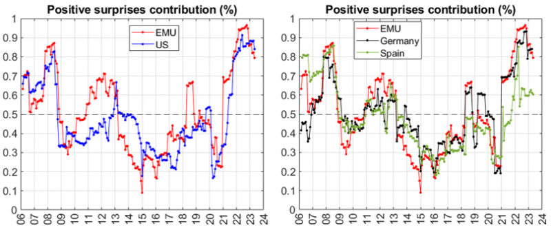
High volatility regimes align with a fast price rise and a rapid price drop. However, we understand that both high-inflation scenarios are different. Is it possible to separate these? The answer is yes. Estimating conditional inflation semi-variances makes it possible to decompose inflation variance into positive and negative surprise components and differ between high volatility related to a fast price rise or drop. This is relevant to understand inflation dynamics’ effects on financial markets and the economy. Figure 4 illustrates the contribution of positive surprises to total inflation variance.7 During the 2022, positive surprises contributed significantly to EMU inflation variance, as expected, as during the GFC and the Sovereign Debt Crisis. The US reached similar positive surprise contributions only during the GFC and since the second half of 2021. It is interesting to confirm the recent reversion of this pattern although the contribution remains at high levels. We recommend to monitor the positive-to-negative surprise contribution to total inflation variance as a way to anticipate changes in the inflation dynamics and trends.