How to set Cyclical and Structural capital buffers via Stress tests? A Risk-to-Buffer approach

This paper proposes a framework to jointly calibrate structural (constant) and cyclical (time varying) bank regulatory capital buffers. Its transparency helps to overcome the risk of omitting or double counting systemic risks when setting capital requirements. This approach consists in producing adverse macroeconomic scenarios whose severity is amplified under high cyclical risk. Risk-related adverse scenarios are fed into stress-tests to assess banks’ losses, should those scenarios materialise. The structural buffer is calibrated using a pre-defined reference risk level. The cyclical buffer is calibrated with respect to the additional losses obtained under the actual current risk level. Our approach is flexible enough to conceptually formalise different calibration approaches and policy preferences, e.g. concerning the choice between setting a positive or a null cyclical buffer in the medium phase of the financial cycle.

Introduction

In reforming bank capital requirements, Basel III regulation introduced the distinction between buffers covering risks associated with the financial cycle (cyclical buffers) and buffers covering structural vulnerabilities (structural buffers). Stress test exercises are key tools for the calibration of those buffers. However, the parallel calibration of those buffers can lead to double-counting or neglecting risks, resulting in over or under-calibration of capital buffers. How to jointly calibrate cyclical and capital buffers via stress test? Our Risk-to-Buffer is a three-step calibration framework solution to this question. First, macroeconomic scenarios are simulated through a non-linear model called Cyclical Amplifier. This model generates adverse scenarios whose severity increases with the level of cyclical risks. Second, scenarios are fed into a Stress test model to project banks capital losses. The harder the macroeconomic scenario, the larger the losses. Third, the losses associated to each scenario are mapped to a buffer. Losses associated to a chosen reference risk level scenario (e.g. the median risk) are used to calibrate the structural buffer. The additional losses associated to the current risk level scenario are used to calibrate the cyclical buffer: when the current risk is higher than the reference risk level, its expected capital losses are larger, and the cyclical buffer is positive. This approach is flexible enough to suit different calibration approaches and policy preferences. One important example concerns the choice between setting a positive or a null cyclical buffer in the medium phase of the financial cycle.

Cyclical buffer and Structural buffers calibration: a Stress test model approach

Since the Global Financial Crisis, prudential authorities and regulators introduced a set of reforms concerning banking regulation (Basel III). One of the novelties of this reform consisted in introducing the distinction between two types of bank capital requirements:

• Counter-cyclical buffer: supposed to move across the financial cycle and cover the build-up of cyclical risks, as such as over indebtedness and asset price over evaluation,
• Structural buffers: constant through the cycle and covering structural risks of the banking system.

The calibration of both types of buffers is a key task of regulators and supervisors. A set of methodologies that became popular to calibrate some of those buffers are Stress test models. Stress tests are a set of equations estimating the evolution of banks’ performance and balance sheet changes under a given macroeconomic scenario. Stress test exercises assess banks’ resilience under adverse scenarios, such as financial crisis or substantial economic downturns. Based on the results of these stress test models, prudential authorities set cyclical and structural requirements: a buffer meant to ensure resilience against a specific risk should cover the estimated losses obtained in case of materialisation. In this way, should the adverse scenario materialize, banks would hold the necessary amount of capital to absorb losses without restricting credit or falling below the minimum requirements.

The parallel use of these exercises for setting both cyclical and structural requirements introduces a risk of overlap: different buffers might end up covering the same type for vulnerabilities. For instance, if structural buffers are set using adverse scenarios whose severity is based on the current financial risk (e.g. high indebtedness), they might incorporate a cyclical component that should instead be covered by cyclical buffers. On the contrary, bad coordination can leave some risks uncovered by calibrated buffers. Finally, it is not clear yet how to calibrate the severity of the scenario and how changes in cyclical risks should be reflected in the degree of scenario severity and, thus, in cyclical buffer calibration.

How to jointly calibrate structural and cyclical buffers? A risk to Buffer approach

How can we jointly calibrate cyclical and structural buffer? Which part of the banks’ capital losses should be covered by a cyclical buffer? Which part should be structurally fixed? How should the cyclical buffer move across the financial cycle?

In order to answer this set of questions, in Couaillier and Scalone (2021) we present a conceptual framework: the ‘Risk-to-Buffer’. This framework is based on the three steps:

1. A non-linear macroeconomic model generates scenarios whose severity increases with the level of cyclical risk; the latter is measured by an indicator of private indebtedness (credit growth, credit over output, etc.)
2. A bank stress test links the macroeconomic scenarios to losses in banks capital ratios.
3. Cyclical and structural ratios are set based on the capital ratios losses. Banks losses obtained under a reference risk scenario are used to calibrate the structural buffer. The additional losses obtained under the cyclical risk scenario are used to calibrate cyclical buffers.

In Figure 1 we provide a conceptual illustration of our approach. Consider that the reference risk level is the historical median risk, the reference risk scenario (yellow line) would be associated to banks losses obtained under this scenario (the sum of the blue and of the yellow bar). If the current risk is larger than the reference risk, so would be the severity of the cyclical risk scenario (red line). The additional losses obtained under this risk scenario (red bar) would be used to calibrate the cyclical buffer.

Figure 1 – Illustrative strategy of buffer calibration by level of cyclical risk

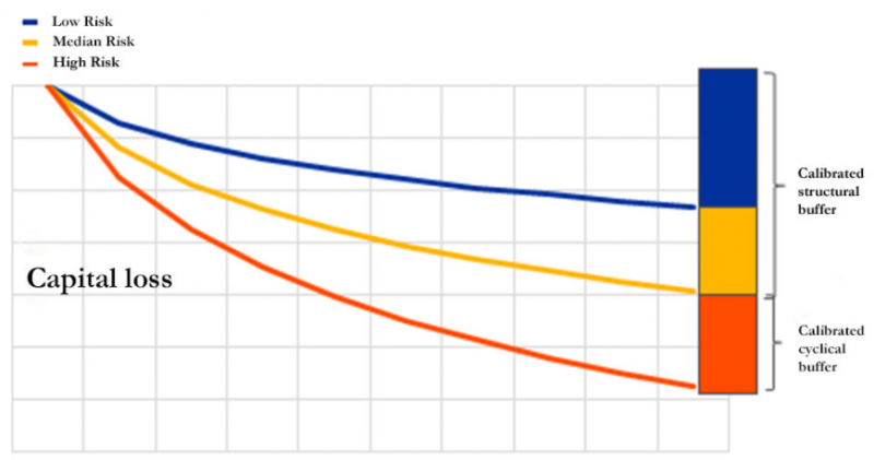
The Risk-to-buffer allows a direct mapping between the level of cyclical risk and the calibrated buffer. For example, should the level of cyclical risk decrease and be included between the high and the reference risk, the cyclical risk scenario would be included between the reference risk and the high cyclical scenario (between the yellow and the red line). According to the Risk-to-Buffer approach, the calibrated cyclical buffer would decrease (a fraction of the red bar). Should the current risk fall below the reference risk, the cyclical buffer would be null, and the structural buffer would act as a backstop on the level of capital buffers.

Which level for the reference risk? A matter of policy preferences

How to set the reference risk for the calibration of the structural buffer is a matter of policy preference. In real life prudential policy, two main approaches exist.

First, some prudential authorities aim at a cyclical buffer at zero in the medium phase of the financial cycle, raising it in the upper phase only. In the Risk-to-Buffer framework, this type of policy preference would mean setting the reference risk at the median risk. As such, the structural buffer would be set equal to banks’ losses projected under the median risk scenario. In this case, the cyclical buffer would be set equal to the difference between the losses obtained under the current cyclical risk and the median scenario losses. It would thus be null for half of the financial cycle and become positive when the cyclical risk is above the median risk.

Other prudential authorities aim at a positive cyclical buffer, e.g. 1%, in normal times. This provides releasable buffers which policymakers could relax in case a crisis hits in a medium risk environment. This type of policy preference is in line with a reference risk fixed below the median, e.g. at the historically minimum level. In such case, the cyclical buffer would be positive as soon as the current risk is higher than the minimum risk. In this alternative calibration, the cyclical buffer would be positive in the medium phase of the financial cycle.

In this sense the Risk-to-buffer does not take a stand on a unique approach (neutral positive or null buffer), but it provides a conceptual framework that can adapt to the policy makers preferences. The relative importance of the cyclical and structural buffers depends on the preference of the policymaker.

A non-linear model to generate Stress test scenario: the Cyclical Amplifier

The central ingredient of the Risk-to-Buffer is the Cyclical Amplifier, a non–linear macroeconometric model generating scenarios whose adversity increases with the level of cyclical risks. As a result, the same shock will produce different effects according to the level of risk in the economy.

In Couaillier and Scalone 2021, we propose a non-linear model estimated on the Euro Area data. We use the Credit to GDP ratio, expressed in 3 years difference, to capture the cyclical risk. First, this measure is one of the most used indicators of cyclical risks. Second, it is a good early warning indicator of the probability and magnitude of future financial crisis (Jorda et al. 2013).

The Cyclical Amplifier can be fed with any set of shocks affecting the variables of the Cyclical Amplifier (e.g. demand shocks, housing shocks and spread shocks). For illustration purpose, we present in Figure 2 the impact of a housing shock, i.e. an exogenous increase in housing prices. This shock can be interpreted as an increase in the demand of housing, bringing to an expansion in housing prices and hence, in collateral prices. We compare the impact of this shock at historically high level (90th percentile of the historical risk distribution) and low level (10th percentile). For the first two years after the shock, when the cyclical risk is high the impact of the housing shock is twice as large as the effect found for the low risk case. On the flip side, it means that a negative housing shock will double its recessionary effect after subdued increase in the credit to GDP ratio: when agents are more indebted, the shock reduces households net wealth and collateral value, pushing down borrowers debt capacity and thus investment and consumption. This type of strong amplification features also other macroeconomic and financial variables considered in our model. A direct implication is the stronger impact of a given shock during the upward phase of the financial cycle.

Figure 2 – Impact of an expansionary housing shock in the Cyclical Amplifier

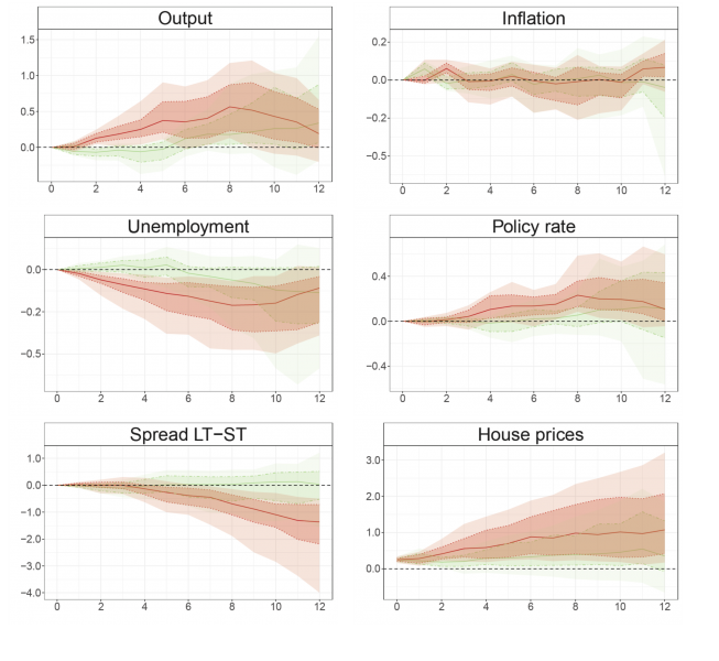
Source: authors’ calculation.
Note: the green (red) line represents the impulse respone function when the cyclical risk is at its 10th (90th) historical percentage; the dark and light colored areas represent the confidence interval at the 67% and 90% confidence interval.

An illustration on European banks: which policy implication for the prudential policy?

In Couaillier and Scalone 2021, we show an illustrative application of the Risk to Buffer on European banks. In our application, macroeconomic scenarios are generated through the Cyclical Amplifier: we consider four different risk levels (Low, Median, High and Max risk, corresponding to the 25th, 50th, 75th and 100th percentiles of historical distribution of our measure).

The set of initial adverse shocks mimics standard EBA Stress test scenario narratives,1 i.e. an asset depreciation, an increase in credit risk and a deceleration of economic activity. This set of shocks is then introduced into the Cyclical Amplifier for the four different risk levels in order to produce four adverse scenarios. As expected, the severity of the scenario increases with the level of cyclical risk.

In a second step we feed these scenarios into a stylised Stress test applied to European banks. Again, the larger the risk, the larger the banks’ projected loss. In the third step, we set the buffers equal to the mean loss across banks triggered by the risk they cover (Figure 3).

Using the median historical risk as the reference level of risk, the structural buffer is set at 3.7% (blue and yellow blocks). The cyclical buffer depends instead on the current level of cyclical risk. If we are currently in a high-risk moment, then the cyclical buffer must cover the orange block, hence 1%. Should the cyclical risk rise to the maximum level, the cyclical buffer would then have to cover both the orange and the brown blocks, rising to 2%.

If instead the policymaker prefers to have more cyclical buffers in normal times, she could calibrate the structural buffer using the low risk scenario. This would put the structural buffer at 1.8% (the blue block). The cyclical risk would then be activated earlier, as soon as the current risk is higher than the historical 25h percentile. At medium risk, it would be at 2% (the yellow block) and at the maximum historical risk at 4% (yellow, orange and brown blocks). As such, setting the reference risk at a lower level provides more releasable buffer but reduces the total buffers in the low phase of the financial cycle.

Figure 3 – CET1 depletion in stress tests (pp) and corresponding buffer(%) for different cyclical risk levels

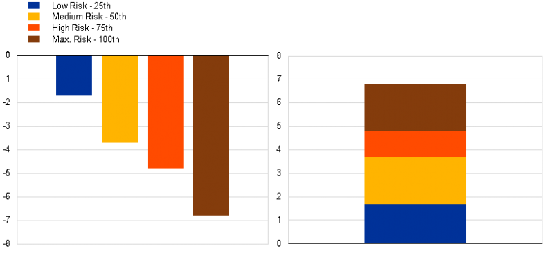
Source: illustrative authors’ calculation.
Note: the left-hand-side panel reports the capital loss in percentage point in the adverse scenario depending on the initial level of cyclical risk (expressed in percentile of historical distribution). The right-hand side panel reports the corresponding buffers.

Conclusion

The Risk-to-Buffer is a transparent and flexible method to jointly calibrate structural and cyclical bank capital buffers. This tool provides a conceptual framework to map risks to buffers. Also, it allows to formally assess how policymaker’s preferences regarding the level of risk at which the cyclical buffer must be activated shape the capital requirements stack. Finally, this approach shows how other prudential measures, as such as borrowers’ based measures, can interact with capital requirements. If a borrower-based measure can decrease private indebtedness, the current cyclical risks will decrease as well. This implies a less severe scenario for the calibration of cyclical buffer, ultimately leading to a lower cyclical buffer reflecting lower cyclical risks.