Inflation shocks and policy delay: what are the consequences of falling behind the curve?

Central banks in major industrialized economies were slow to react to the surge in inflation that began in early 2021and have since faced difficulty taming persistent inflation. We evaluate the consequences of such a delay in responding to a temporary but persistent positive shock to inflation. Policy delay worsens inflation outcomes but can mitigate or even reverse the output decline that occurs when policy responds without delay; consequently, delay can make a recession less likely. Using a measure of loss that incorporates a “balanced-approach” to weighing fluctuations in inflation and the output gap, our research finds that loss is monotonically increasing in the length of the delay. Loss is reduced if policy, when it does react, does so more aggressively. The costs of a short delay can be eliminated by adopting a less inertial and more aggressive response to inflation.

2021 provided vivid evidence of how large shocks to aggregate demand and supply can lead to sharp surges in inflation. The view that the rise in inflation was the result of temporary factors, combined with confidence that ten years of low inflation had firmly anchored inflation expectations, led central banks to believe inflation would quickly return to pre-COVID levels. As a consequence, many central banks, including the Federal Reserve, the Bank of England, and the European Central Bank, delayed responding as inflation rose well above the banks’ official targets. In the U.S., the Federal Reserve raised its policy rate only in March 2022, a year after PCE inflation had breached its 2-percent target.

Standard analyses of monetary policy assume that central banks react immediately when shocks occur; the consequences of waiting to react, as central bankers did in 2021 and early 2022, are not well understood. The slow reaction to inflation during 2021 raised several important questions: How costly is delay when fighting a surge in inflation? If a policy is delayed, should it then be more aggressive? Is a credible promise to eventually fight inflation a substitute for undertaking immediate action? In a recent paper (Hakamada and Walsh (2024)), we address these questions by evaluating the consequences of waiting to respond to a surge in inflation.

The standard policy prescription in the face of a rise in inflation is to boost the policy rate to raise the real interest rate, leading to a contraction in demand that moderates the initial rise in inflation. However, when policy fails to react, a surge in inflation that is expected to persist produces a fall in the real interest rate, as expected inflation increases and the nominal policy rate remains unchanged. This decline in the real rate stimulates aggregate demand and boosts output, exacerbating rather than dampening the rise in inflation.1 Two conclusions follow. First, delay affects inflation and the output gap differently. Greater delay leads to higher inflation but also a smaller decline and potentially even a rise in the output gap. Second, if policy outcomes are evaluated using a standard quadratic loss function in inflation and output gap volatility, the loss caused by policy delay will depend critically on the weight placed on economic activity relative to inflation stability. If that weight is large, delay may be preferred to responding immediately; if the weight is small, delay will be costly.

Delay in a new Keynesian model

To investigate the effects of policy delay, we employ a simple new Keynesian model. The model includes several sources of persistence: habits in consumption, inertia in the central bank’s policy rule, and serial correlation in the inflation shock. We adopt standard values for the calibrated parameters from Galí (2015). For the policy rule, we assume a basic Taylor rule with inertia. Our baseline rule sets coefficients of 1.5 on inflation and 0.5 on the output gap when inflation is expressed at annual rates. Policy inertia, reflected in the coefficient on the lagged policy rate, is set to 0.85. The size of the inflation shock innovation is calibrated to generate a peak rise of quarterly inflation over target of 9 percent (expressed at an annual rate) when policy delays four periods before reacting. This delay corresponds to the year the Fed waited before reacting. We set the AR(1) coefficient for the inflation shock process at 0.85.

In Hakamada and Walsh (2024), we considered policy delays, denoted by k, of zero (an immediate reaction) to 6 quarters, but here we focus on two cases: no delay (k = 0) and a one-year delay (k = 4). To represent a more aggressive policy response, we double the coefficient on inflation in the policy rule, denoted by ϕ_π, to 3.0. An aggressive policy response can also be interpreted as a rule with less persistence, so we also consider the effects of reducing policy inertia from 0.85 to 0.5.

Figure 1 illustrates the responses of the nominal policy rate, the real rate, the output gap and inflation to the inflation shock. The black lines are obtained when policy reacts immediately to the shock; the blue lines show the effects of waiting four-quarters to react. The responses with the baseline instrument rule in which ϕ_π = 1.5 are shown by the solid black lines. When the policy response is immediate, inflation rises, but by less than 4%. The cost is a prolonged but mild recession with the output gap falling less than 1% at its trough. The blue solid lines show the responses when the central bank delays for 4 quarters before reacting. In this case, inflation peaks at 9%. However, the sharp rise in inflation, combined with no change in the nominal policy rate, implies a large decline in the real interest rate. This leads to a strong economic expansion, results consistent with the explanation of delay’s effects outlined above.

Figure 1: Response to an inflation shock with and without a delayed policy response
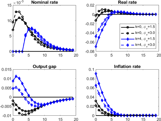Notes: The figure reproduces results from Hakamada and Walsh (2024). The black (blue) solid lines with filled circles (diamonds) show the impulse responses to the inflation shock when policy reacts immediately (with a four-quarter delay) with a coefficient on inflation in the policy rule of 1.5. The responses with dashed lines and open circles (diamonds) are obtained when the coefficient on inflation in the policy rule is 3.0.

Does delay call for a stronger response to inflation once policy does act?

This question was raised during 2022 as the Fed began lifting its policy rate, and the FOMC embarked on a series of rate increases that were larger than its normal practice of moving in 25-basis point increments. While the first move in March 2022 was a 25-basis point increase, this was followed by a 50-basis point hike in May 2022. Four further increases of 75 basis points followed.

We consider two interpretations of a more aggressive policy response. The first interpretation treats an aggressive policy as one that assigns a larger value to ϕ_π, the coefficient on inflation in the policy rule. The second interpretation views a more aggressive policy as one that assigns a smaller weight ρ_i to lagged inflation and that, therefore, displays less inertia. The contemporaneous response of the policy rate to inflation is equal to (1 −ρ_i)ϕ_π, which increases with a rise in ϕ_π, (i.e., a stronger response to inflation) or a fall in ρ_i, (i.e., less inertia).

The dashed lines in Figure 1 show the impulse responses under a more aggressive policy in which the response coefficient on inflation is doubled to 3.0. This more aggressive response dampens the rise in inflation regardless of delay, but it also reduces the path of the output gap. This means that the recession when the central bank reacts immediately is worsened, while a 4-quarter policy delay still generates an initial expansion in economic activity, though a smaller one than with the baseline, less aggressive policy rule.

The more aggressive policy reduces deviations of inflation from its target. Whether the behavior of the output gap is improved is less obvious. With k = 0, the more aggressive response to inflation leads to larger deviations of the output gap from zero. Aggression is not clearly better when k = 0: inflation performance is improved; output gap performance is worsened.

In contrast, when the central bank fails to respond quickly, when it does act, it should respond aggressively. As the figure shows, when k = 4, inflation performance improves when ϕ_π = 3.0, while the discounted deviations of the output gap from zero fall.

The second definition of a more aggressive policy is to act with less inertia. We find that with the baseline coefficient of 1.5 on inflation, reducing the coefficient on the lagged policy rate from 0.85 to 0.5 leads to a much larger rise in the nominal rate, both initially and throughout the convergence back to steady state. This is also the case when k = 0 and k = 4. Less inertia front-loads the interest rate increase. Absent any policy delay, the less inertial policy rule produces a higher real interest rate path and has a small effect in lowering the path of the output gap. The effect on inflation of the less inertial policy is small, but when k = 0, the less inertial, more aggressive policy does contribute to dampening inflation.

Ranking outcomes

Because different policy rules and changes in the extent of delay can affect inflation and the output gap differently, we need a metric to evaluate outcomes. The normal approach in the literature using linear new Keynesian models is to employ a weighted sum of the variance of inflation and the variance of the output gap. This is appropriate when considering a stochastic equilibrium in which the economy experiences new shocks each period. Our objective, however, is to understand how the choice of delay affects the response to a single inflation shock realization.

We therefore rank outcomes by using a loss metric defined as the average squared deviations of inflation and the output gap as a function of the time since the shock. The weight on output deviations relative to inflation deviations is obtained using a using a balanced-approach that assumes deviations of inflation and the unemployment rate from target are given equal weight. We then use Okun’s Law with a coefficient of 2 to translate fluctuations in the unemployment rate into fluctuations in the output gap.

We evaluate loss for four policy rules that differ on whether the response coefficient to inflation ϕ_π is weak (1.5) or strong (3.0) and inertia ρ_i is high (0.85) or low (0.5). Results are reported in Figure 2, taken from Hakamada and Walsh (2024).

The figure shows the average weighted volatility of inflation and the output gap as a function of time since the shock. Each panel shows results for different values of the policy response to inflation and the degree of policy inertia. The policy response begins in period k. The upper left panel uses our baseline policy rule, while the lower right panel is the most aggressive rule. The vertical scale differs across panels.

Figure 2: Loss as a function of the policy rule and delay

Notes: This figure, taken from Hakamada and Walsh (2024) shows average cumulative loss as measured by a balanced-approach quadratic loss measure. The horizontal axis means time since the shock, and k is the number of periods before the central bank reacts. Note the vertical scales differ across panels.

Across all four panels, loss is increasing with delay at each horizon. There is also a clear ranking of the policy rules. Worst is the baseline rule based on the Taylor rule coefficients and a common empirical estimate of policy inertia (upper left). The next best rule employs the same response coefficient but with less inertia (lower left). Even better is the rule with a strong response to inflation and the same degree of inertia as the baseline rule (upper right). Finally, the rule that results in the lowest loss at each horizon and for each k is the most aggressive one that combines a strong response to inflation and less inertia (lower right).

Can aggressiveness compensate for falling behind the curve?

To answer this question, we compare the loss under our baseline policy that reacts immediately to the shock with policies that are implemented with delays of 1 to 4 quarters and that adopt the most aggressive policy rule (corresponding to the rule in the lower right panel of the previous figure). Results are shown in Figure 3.

Loss is lower at each horizon with a one period delay and an aggressive policy rule. The baseline loss (with k = 0) is replicated with a two-period delay and an aggressive rule. Any further delay leads to worse outcomes than the baseline policy. Thus, aggression can compensate for delay, but only if the delay is relatively short.

Figure 3: Loss and Expectations

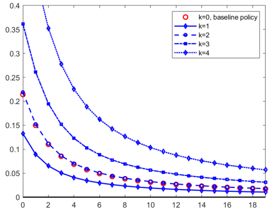
Notes: The red circles show our measure of loss as a function of time since the shock.

Do results depend on the power of forward guidance?

The results discussed so far assumed rational expectations, implying that the public knows the central bank’s rule and knows that the central bank will eventually react in the future. The literature on forward guidance finds that beliefs about what the policy authority will do in the future can have large effects immediately. In Hakamada and Walsh (2024), we investigated how the costs of delay are affected when forward guidance is less powerful. Adopting the cognitive discounting model of Gabaix (2020), we found that both inflation and the output gap are less volatile when agents display cognitive discounting as expectations of the future play a smaller role. However, the general conclusions obtained under rational expectations still held: Loss was lowest when there is no delay in responding, and conditional on delay, loss was lower when policy reacts more aggressively.

Lessons

Our results show that policy delay worsens inflation outcomes but can mitigate or even reverse the output decline that occurs when policy responds immediately, an important consideration when policymakers are particularly concerned with preventing a recession.

We find that delay increases peak inflation and, by reducing the real interest rate, initially leads the output gap to rise, Delay mitigates subsequent declines in the output gap during the adjustment back to steady state. This produces a trade-off: reacting more quickly depresses economic activity but helps dampen the rise and persistence of inflation.

When fighting a surge in inflation, loss is minimized when policy responds without delay. However, delay is not very costly if the delay is only one or two periods; it can be much more costly if delay extends to four periods or longer.

If policy is delayed, it should be more aggressive. We explored the implications of two definitions of a more aggressive policy response. The first definition focuses on the inflation coefficient in the policy rule; the second focuses on the degree of inertia in the policy response. A more aggressive policy is one that places a larger coefficient on inflation or displays less inertia. Conditional on falling behind the curve, loss is smallest when policy reacts strongly to inflation and with less inertia.

Finally, a credible promise to fight inflation in the future can substitute for undertaking current policy actions, but only if the delay is short and the future response is aggressive. This suggests that policymakers who do fall behind the curve need to be more aggressive when they finally do react.