menu
close

Author(s):

Sandra Daudignon | Ghent University
Oreste Tristani | European Central Bank (ECB)

Keywords:

nonlinear optimal policy , zero lower bound , commitment , liquidity trap , New Keynesian

JEL Codes:

C63 , E31 , E52
Empirical analyses starting from Laubach and Williams (2003) find that the natural rate of interest is not constant in the long-run. This paper studies the optimal response to stochastic changes of the long-run natural rate in a suitably modified version of the new Keynesian model. We show that, because of the zero lower bound (ZLB) on nominal interest rates, movements towards zero of the long-run natural rate cause an increasingly large downward bias in expectations. To offset this bias, the central bank should aim to keep the real interest rate systematically below the long-run natural rate, as long as policy is not constrained by the ZLB. The neutral rate – the level of the policy rate consistent with stable inflation and the natural rate at its long-run level – will be lower than the long-run natural rate. This is the case both under optimal policy, and under a price level targeting rule. In the latter case, the neutral rate is equal to zero as soon as the long-run natural rate falls below 1%. 

1. Introduction

Although monetary policy rates have increased rapidly in recent quarters, in response to the rise in energy prices and inflation, it can be expected that price stability will be restored in the medium term. At that point, monetary policy rates will return to their neutral level – the level consistent with stable inflation and the real rates at their long-run, natural level.  Empirical estimates suggest that the long-run natural rate has drifted towards values close to zero in recent decades, and is expected to remain low for quite some time. For example, Holston et al. (2017) finds that, in 2016, the long-run natural rate was around 0.5% in the US and possibly slightly negative in the Euro Area. The future evolution of the long-run natural rate is also uncertain. Platzer and Peruffo (2022) forecast the natural rate in the US to reach a trough of 0.38% by 2030, and then rise again to 1% in the very long run. How is the neutral policy rate affected by the expected, low value of the long-run natural rate, given the zero lower bound on nominal rates? What is the optimal conduct of monetary policy in view of the prevailing uncertainty as to the future level of the long-run natural rate?

2. A new Keynesian model: distinctive features, solution method, and calibration

We study these questions in the context of a new Keynesian model with transitory natural rate shocks (due to changes in consumer taste), permanent natural rate shocks (due to changes in the productivity trend growth rate), and sticky prices à la Calvo. The model is able to replicate the empirical features of the long-run natural rate in recent years, as reported in the empirical literature. It also takes into account the zero lower bound (ZLB) on nominal interest rates.1
More specifically, the model economy has two distinctive features. First, the trend productivity growth rate follows a unit root process over a bounded support. The unit root assumption reflects our uncertainty as to the evolution of productivity growth in the distant future. The boundaries capture the idea that extremely high, or negative, long-run growth rates for productivity are implausible. The boundaries induce some reflecting behavior in the productivity growth rate, which can only decrease (increase) after reaching the upper (lower) bound. This assumption is consistent with estimates of the trend productivity growth rate which fluctuate within a narrow, positive range in the period following World War II. In the model, permanent shocks to the trend productivity growth rate induce time-variation in the long-run natural rate. The second distinctive feature of our model is that households derive utility from their holdings of Treasury bonds (Fisher 2015, Krishnamurthy and Vissing-Jorgensen 2012, Michaillat and Saez 2021). This assumption captures the idea that government bonds have special, liquidity value relative to other assets, and they therefore incorporate a convenience yield. In our model, the assumption has the benefit of allowing for interest rate levels very close to zero, even if productivity growth remains positive. The model solution is based on projection methods and accounts for the nonlinearity induced by the ZLB. The solution is stochastic. We can therefore study the effects on the solution of the mere risk of unexpected future changes in the natural rate of interest.
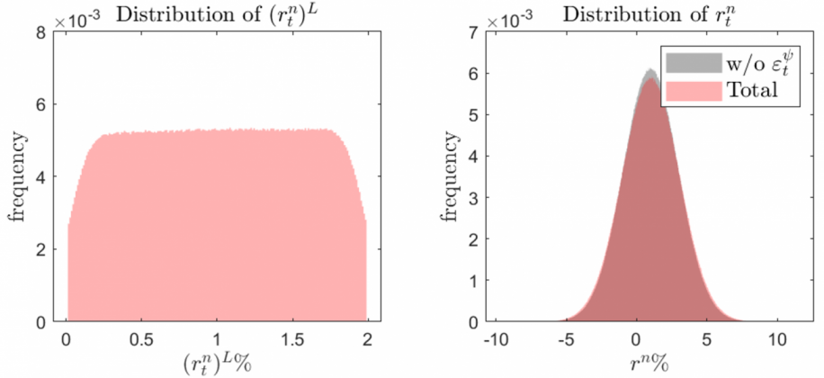
Figure 1: Unconditional distribution of the natural rate
 width=
Notes: Both the long-run natural rate (left panel) and the natural rate with or without permanent shocks to the productivity trend growth rate (right panel) are expressed in annualized terms. 
Source: Daudignon and Tristani (2023). 

Compared to the benchmark new Keynesian model, four new parameters emerge: the boundaries and the standard deviation of shocks to the trend productivity growth rate, and the convenience yield on treasuries. For the productivity trend growth rate, we set the value range between 1% and 3% and the standard deviation of shocks to about one tenth that of transitory real rate shocks. This reflects both the value range that we obtain for the US economy and the value range that Holston et al. (2017) obtain for the Euro Area. The standard deviation is based on the estimate in Fiorentini et al. (2018), which uses historical data for a set of 17 economies. Finally, the subjective discount factor and the convenience yield are calibrated so as to replicate the features of the long-run natural rate in recent years, i.e., to drift towards values around zero. For the convenience yield on treasuries, we follow Del Negro et al. (2017), which finds that it might have reached 3% in the US in 2016. For the subjective discount factor, we follow Platzer and Peruffo (2022) which forecasts a natural rate of 1% in the US in the very long run.

3. Monetary policy ought to be over-expansionary at low levels of the long-run natural rate

The first experiment focuses on the optimal conduct of monetary policy. As in the rest of the new Keynesian literature, we assume that the only tool available to the central banker is the short-term interest rate, and that her commitment regarding future policy is perfectly understood by the public and fully credible.
The central banker chooses the state-contingent path that maximizes the second order approximation of aggregate welfare, which is a concave function of current and future detrended output gaps and inflation rates, subject to agents’ optimal decisions, which in reduced form are represented by a Phillips and IS curve. As usual, absent the lower bound on the policy rate, shocks – whether transitory or permanent – would not justify any fluctuations in output and prices. The central banker should maintain output at potential and stable prices by setting the policy rate equal to the natural rate at any point in time. Due to the lower bound on nominal interest rates, however, it is impossible to set the policy rate equal to the natural rate when the latter turns negative. In these contingencies, periods of below-potential output and deflation are inevitable. The likelihood of temporarily negative natural rates increases when the long-run natural rate is very low and close to zero. The mere risk that the lower bound may be hit in the future will be reflected in private sector’s expectations. The central banker may then want to act preemptively and ease the monetary policy stance.
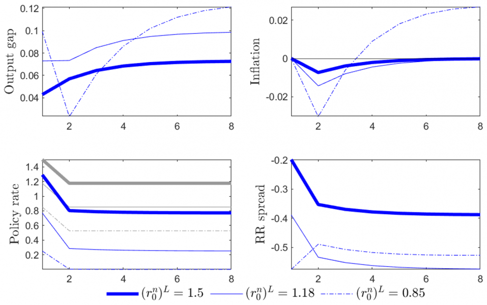
Figure 2 displays the optimal outcome following a large negative permanent shock to the long-run natural rate in isolation, starting from different initial values of the long-run natural rate. The figure shows that the shock affects the risky steady state of the economy, that monetary policy should be over-expansionary relative to the case without the ZLB, and that the strategy depends on the initial value of the long-run natural rate.
Figure 2: Impulse responses to permanent shocks under optimal policy
 width=
Notes: The figure shows impulse responses to permanent shocks of a given size (0.324 p.p., i.e., three times the standard deviation of permanent real rate shocks) starting from different values of the long-run natural rate. The grey lines in the policy rate panel indicate the natural rate. The response of the output gap is in p.p.; all other responses are expressed in annualised p.p.. Source: Daudignon and Tristani (2023).
The bottom left panel in Figure 2 shows the paths of the policy rate and the natural rate following the shock. After 8 quarters, the policy rate reaches its new long-run level, i.e. the neutral rate. The panel demonstrates that, starting from values equal to 1.5% or 1.18%, the neutral rate should fall more than proportionally to the decline in the long-run natural rate, the more so the closer the long-run natural rate falls towards zero. The non-linear relationship between the long-run natural and the neutral rate is driven by an expectation effect. Everything else equal, the lower the long-run natural rate, the lower the policy rate consistent with potential output (IS curve) and with price stability (Phillips curve). But, a lower policy rate also reduces the scope for monetary policy easing in the face of possible adverse shocks, which amplifies the downside bias in expectations due to the ZLB. A one-to-one adjustment in the policy rate is therefore not enough to stabilize output and inflation. The gap between the neutral rate and the long-run natural rate should be negative and tailored to produce a positive output gap that is large enough to offset the deflationary bias in inflation expectations. The policy rate adjusts slowly to its neutral value. This policy ensures that price stability is restored, after a short-lived deflationary episode.

Outcomes change for lower initial values of the long-run natural rate. Figure 2 illustrates the case when this is equal to 0.85% and the initial value of the neutral rate is slightly larger than 0.2%. The policy reaction described above is no longer feasible due to the lower bound. In the new risky steady state, the neutral rate reaches zero, but this amount of easing is insufficient to offset the deflationary bias in expectations. The central banker mitigates the deflationary bias by committing to create inflation and an output boom in reaction to future positive shocks. This promise exerts an expansionary effect on both actual output (IS curve) and actual inflation (Phillips curve) and translates into positive actual inflation.

4. Price-level targeting: a feasible way to approximate the optimal outcome in practice

The second set of experiments focuses on the extent to which a simple price level targeting rule can replicate the optimal outcome.
This type of rule is a good candidate because it does not require any estimate or knowledge of the long-run natural rate, which is difficult to filter from the data, especially in real time. Moreover, we already know from the work of Eggertsson and Woodford (2003) that it performs well when the natural rate in normal time hovers around 4%. More specifically, they show that optimal policy can be described as a gap-adjusted log price level (GAPL) target. They also put forward a simpler version of the rule, where the price level target is constant over time. When perfect inflation stabilization is not feasible because of the ZLB, the rule ensures that deflationary episodes are followed by periods of positive inflation, so as to ultimately bring the GAPL back to target.
Figure 3: Welfare loss under price level targeting with drift
 width=
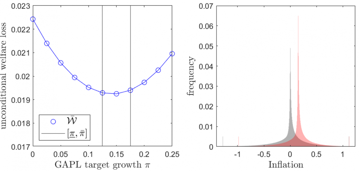
Notes: The left panel shows the welfare-theoretic loss function for different values of the GAPL target growth. The right panel shows the unconditional distribution of inflation winsorized at 1% under price level targeting when the GAPL target growth is equal to zero (grey) and to the optimal value of 15 basis points (red). Both the GAPL target growth and the inflation rate are expressed in annualized percentage terms. Source: Daudignon and Tristani (2023).
An obvious generalization of the simple Eggertsson and Woodford (2003) rule is to allow for an exogenous deterministic trend in the target price level. The exogenous value of the trend can then be set so as to maximize aggregate welfare. The advantage of the generalized Eggertsson and Woodford (2003) rule is to increase the neutral rate and thereby increase the scope for lowering the policy rate in reaction to adverse shocks. Its disadvantage is to always allow for positive inflation, which is costly for the economy.
Comparing welfare losses across rules, we obtain two results. First, a growing price level target yields marginally superior outcomes. The left panel of figure 3 displays the value of the unconditional welfare loss under different calibrations of the GAPL target growth. It shows that a growing target is preferable to a constant target as long as the target growth does not exceed 25 basis points, and that the optimal target growth lies around 15 basis points. However, in relative terms, the welfare loss under the constant target is only about 17% larger than the welfare loss under the optimal simple GAPL target. Second, this type of simple price level targeting rule continues to perform well in the sense that the welfare loss under the optimal simple GAPL target is only 64% larger than the welfare loss under optimal policy.
Figure 4: Impulse responses to a sequence of permanent shocks under various rules
 width=
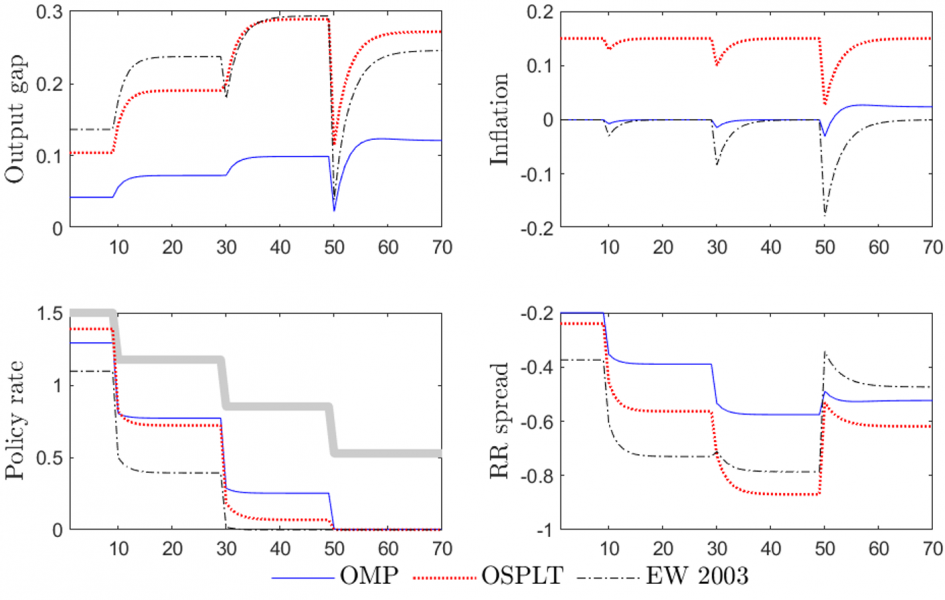
Notes: The figure shows the results of the simulation of a sequence of three negative permanent shocks to the long run natural rate. Starting from a value equal to 1.5% at time 0, it falls successively by 0.324 p.p., i.e., three times the standard deviation of permanent real rate shocks, at time 10, 30, and 50. Following this sequence of shocks, the long run natural rate is equal to 0.528%. In each panel: the solid blue line indicates outcomes under the optimal policy; the dotted red and black lines indicate outcomes under the optimal and constant simple price-level targeting rules respectively. The solid grey line in the policy rate panel indicates the natural rate. The response of the output gap is in p.p.; all other responses are expressed in annualized p.p.. Source: Daudignon and Tristani (2023).

Figure 4 displays impulse responses to a sequence of three large negative permanent shocks to the long-run natural rate, which bring it from 1.5% to 0.5%, under optimal policy (blue), the constant price level targeting rule of Eggertsson and Woodford (black dotted line), and the optimal simple price level targeting rule (red). It shows that the neutral policy rate reaches zero earlier under price level targeting than under optimal policy. For the constant price level targeting rule, this is the case already when the long-run natural rate falls below 1%. This is due to the fact that simple rules are less sophisticated than optimal policy in their ability to manage expectations in reaction to adverse shocks. When the economy contracts and the GAPL undershoots the target, optimal policy prescribes to increase the target by an amount proportionate to the actual target shortfall, which commits the central bank to conduct a more expansionary policy in the future than what is needed to undo deflation. By contrast, under simple rules, the target is exogenous. A constant target for example would commit the central bank to “just” undo deflation. This policy is less effective in mitigating economic contractions. For a given value of the long-run natural rate,  the negative skew in expectations induced by the ZLB constraint is therefore larger, the output gap needed to offset the deflationary bias in inflation expectations is higher, and the neutral policy rate is lower.

5. Concluding Remarks

Empirical research suggests that the long-run natural interest rate is not constant, but time-varying. Accounting for this empirical feature in a simple new Keynesian model, we have shown that the risk of future reductions in the long-run natural rate tends to impart a downward bias on output and inflation expectations. To offset this bias in expectations, a central banker should aim to maintain the policy rate below the natural rate as long as this approach is feasible – i.e. until the policy rate hits its lower bound. Nearly optimal outcomes can be achieved through price level targeting rules, especially if they incorporate a small exogenous drift in the price level.

References

Daudignon, S., & Tristani, O. (2023). Monetary policy and the drifting natural rate of interest. ECB Working Paper.
Del Negro, M., Giannone, D., Giannoni, M. P., & Tambalotti, A. (2017). Safety, liquidity, and the natural rate of interest. Brookings Papers on Economic Activity, 2017(1), 235-316.
Eggertsson, G. B., & Woodford, M. (2003). Zero bound on interest rates and optimal monetary policy. Brookings papers on economic activity, 2003(1), 139-233.
Fiorentini, G., Galesi, A., Perez-Quiros, G., & Sentana, E. (2018). The rise and fall of the natural interest rate. Banco de Espana Working Paper 1822.
Fisher, J. D. (2015). On the Structural Interpretation of the Smets–Wouters “Risk Premium” Shock. Journal of Money, Credit and Banking, 47(2-3), 511-516.
Holston, K., Laubach, T., & Williams, J. C. (2017). Measuring the natural rate of interest: International trends and determinants. Journal of International Economics, 108, S59-S75.
Krishnamurthy, A., & Vissing-Jorgensen, A. (2012). The aggregate demand for treasury debt. Journal of Political Economy, 120(2), 233-267.
Laubach, T., & Williams, J. C. (2003). Measuring the natural rate of interest. Review of Economics and Statistics, 85(4), 1063-1070.
Michaillat, P., & Saez, E. (2021). Resolving New Keynesian anomalies with wealth in the utility function. Review of Economics and Statistics, 103(2), 197-215.
Platzer, J., & Peruffo, M. (2022). Secular Drivers of the Natural Rate of Interest in the United States: A Quantitative Evaluation. IMF Working Paper No. 2022/030.

  • 1.

    The euro area experience has demonstrated that the effective lower bound on nominal interest rates is not zero, but somewhat negative due to cash storage costs. We abstract from this feature in our simple model.

About the authors

Sandra Daudignon

Sandra Daudignon is a Post-doctoral researcher and lecturer at Ghent University. She holds a Ph.D. in Economics from the Paris School of Economics and from the University of Paris 1 Panthéon-Sorbonne.

Oreste Tristani

Oreste Tristani is a Senior Adviser in the Directorate General Research, European Central Bank and a Research Fellow of the Centre for Economic Policy Research (CEPR).

More on these topics

Tags: