Reconciling Random Walks and Predictability: A Dual-Component Model of Exchange Rate Dynamics

Abstract
Many economists assume that exchange rates follow a random walk, as statistical tests show that exchange rates do not exhibit mean reversion. But survey data show that expected exchange rate changes are not zero and have an inverse link with the exchange rate level. We reconcile this puzzle by showing that exchange rates combine a random unpredictable trend with a predictable cyclical component. Using data from nine advanced economies (2000-2024), we show that expected one year exchange rate changes have considerable predictive power for subsequent multi-year changes, with the predictive power increasing as the forecast horizon widens. Our model also improves forecast accuracy by up to 49% compared to a random walk over medium-term horizons.

1. Introduction

A key question in international finance is whether exchange rates are predictable or follow a random walk. If exchange rates are stationary, they revert to a long-term average, meaning that a high exchange rate today suggests depreciation in the future. By contrast, if exchange rates follow a random walk, their future level is unpredictable and best approximated by today’s level.

Economists often use statistical tests, such as the Augmented Dickey Fuller (ADF) test and the KPSS (Kwiatkowski-Phillips-Schmidt-Shin) test, to determine whether exchange rates are stationary. The ADF test examines whether a time series has a unit root (indicating absence of mean reversion), while the KPSS test assumes stationarity (mean reversion) as its starting point.

Applying these tests to monthly exchange rate data for 2000-2024 from nine advanced economies with freely floating currencies, we find consistent results: exchange rates are not stationary. The ADF test fails to reject the presence of a unit root, while the KPSS test rejects stationarity.

2. Why Exchange Rates Combine a Stationary Component with a Slowly Moving Trend

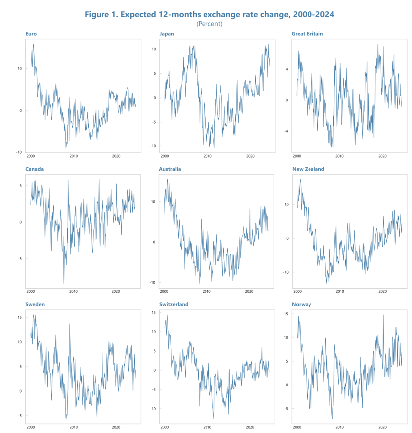
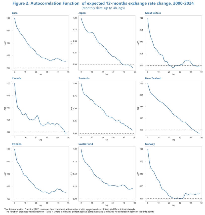
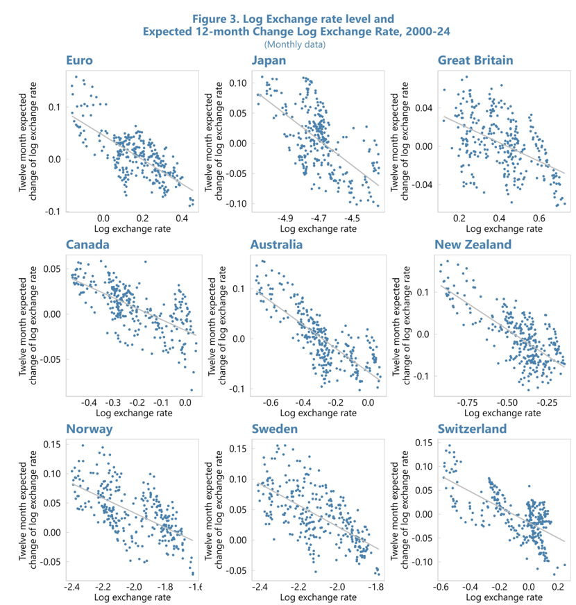
If exchange rates followed a pure random walk, the best guess for next year’s exchange rate would always be today’s rate. However, reality tells a different story. Looking at survey data from 2000-2024 of what investors expect exchange rates to do over the next 12 months, we see three important patterns: 1

• Expected exchange rate changes are not zero and can be quite large (Figure 1).
• These expected changes persist – if investors this month expect the currency to strengthen over the next 12 months, they usually expect similar changes next month (Figure 2).
• When exchange rates are high, investors tend to expect them to fall, and vice versa (Figure 3)

This creates a puzzle: statistical tests show exchange rates have a “unit root” (suggesting that they follow a random walk and expected exchange rate changes should be zero), yet market participants consistently expect non-zero changes.

In a recent paper (Bakker (2024)) I show that the solution lies in viewing exchange rates as having two parts: a slow-moving random trend that can’t be predicted (a “random walk”), and a cyclical component that tends to return to normal level.

To understand how this works, imagine a currency appreciates by 20%. Consider two scenarios:

• In the first scenario, most of the appreciation—90%, or 18 percentage points—is due to the cyclical component, while only 2 percentage points are attributable to the trend. In this case, the prediction is that the currency will likely depreciate by approximately 18% in the medium term as the cyclical component reverts to its normal level.
• In the second scenario, the situation is reversed: 90% of the appreciation—18 percentage points—is driven by the trend, while only 2 percentage points come from the cyclical component. Here, the prediction is that the currency will likely depreciate by only 2% in the medium term, as most of the appreciation reflects a permanent change in the equilibrium exchange rate.

In the first scenario, most of the exchange rate shocks are reversed, and there is considerable medium-term predictability. In the second scenario, little of the exchange rate shocks are reversed and there is little medium-term predictability.

These scenarios demonstrate a crucial insight: the relative size of the trend versus cyclical components determines how predictable future exchange rate movements will be. When changes are mostly cyclical, we can predict substantial reversals. When changes are mostly driven by permanent shifts in the equilibrium exchange rate, we expect little reversal. This framework explains why expected exchange rate changes aren’t zero: unless the cyclical component happens to be zero, investors will always expect some movement as the cyclical part returns to normal levels. The size of the expected change depends on how far the cyclical component has deviated from its normal level.

Next, we explain why the stochastic trend must be moving slowly. This is so for two reasons: if it were not, expected exchange rate changes would not be highly persistent, and there would not be a strong link between exchange rate levels and expected exchange rate changes.

The persistence of expected exchange rate changes is influenced by the persistence of the cyclical component, which varies depending on whether exchange rate changes are driven primarily by the stochastic trend or by the cyclical component. If exchange rate changes are largely influenced by the cyclical component, the stochastic trend will evolve slowly, resulting in potentially large and persistent expected changes. If the stochastic trend drives most of the exchange rate changes, the cyclical component will remain small, leading to relatively small and less persistent expected changes.

Note that while the cyclical component generates medium-term predictability, in the long-term exchange rates are unpredictable due to the presence of the random walk.

In sum, we can explain the three observations (a) exchange rates have a unit root; (b) expected exchange rate changes are highly persistent; (c) there is a strong link between exchange rate levels and expected exchange rate changes by assuming that exchange rates combine a slowly moving stochastic trend with a stationary component.

3. A Model of the Stationary Component

To move from theory to practice, we need to understand what drives the stationary component. This paper uses the Bachetta and van Wincoop (2021) framework for the stationary component.

The Bachetta and van Wincoop (2021) model shows how exchange rates respond to interest rate differentials when investors are risk-averse, and portfolio adjustment is gradual. When one country’s interest rates exceed another’s, its currency tends to appreciate as investors seek higher yields. However, because investors adjust their portfolios gradually and are sensitive to risk, this appreciation occurs over time rather than instantly.

How Interest Rates Drive Mean Reversion

Interest rate differentials themselves tend to be mean-reverting. When a country’s interest rates rise above its trading partners, its currency appreciates as investors are attracted by the higher yields. However, over time, interest rates between countries tend to converge. As the interest rate gap narrows, the exchange rate naturally moves back toward its equilibrium level. This creates a predictable pattern of exchange rate movements over the medium term, even though short-term movements may appear random.

Economic Foundations

This mean reversion in interest rates and exchange rates is rooted in how central banks respond to economic conditions. When an economy overheats and operates above potential, the central bank raises interest rates. This higher interest rate attracts foreign capital, leading to currency appreciation.

However, the higher interest rates eventually cool the economy, allowing rates to fall back toward normal levels. As interest rates normalize, the currency weakens.

The opposite occurs during economic slowdowns. When an economy operates below potential, the central bank lowers interest rates, causing the currency to depreciate. These lower rates help stimulate recovery and, as the economy strengthens, interest rates rise again and the currency strengthens.

These patterns become particularly pronounced when two economies are at different points in their cycles. Consider two countries experiencing opposing economic conditions – one overheating while the other faces a slowdown. The country with strong growth raises rates while the other keeps them low, creating a substantial interest rate differential and exchange rate movement. However, as the overheating economy cools and the weak economy recovers, interest rates converge. This convergence in interest rates drives the exchange rate back toward its equilibrium level.

4. The Predictive Power of Expected One-Year Exchange Rate Changes

Thus, while exchange rates contain an unpredictable random walk component that dominates in the long run, the stationary component creates systematic patterns over the medium term through these fundamental economic mechanisms. These mechanisms ensure that when exchange rates deviate substantially from equilibrium – whether through interest rate changes or other factors – they tend to revert over time.

In the short term, exchange rate changes are predominantly driven by stochastic shocks rather than systematic mean reversion. This makes short-term exchange rate predictions particularly challenging. Conversely, as the time horizon extends, mean reversion becomes increasingly pronounced, enhancing the predictability of exchange rate changes.

Theoretically, this suggests that longer-term exchange rate forecasts should demonstrate superior predictive power compared to short-term predictions. The strength of mean reversion intensifies with the forecast horizon. Unfortunately, we cannot test this hypothesis as we only have one-year expected exchange rate changes.

However, we can find a proxy for expected multi-year changes. Because exchange rate adjustment is gradual, expected changes over longer periods are larger than expected one-year changes. For instance, the expected two-year change is larger than the expected one-year change, and the expected three-year change is larger than the expected two-year change. This implies that the expected multi-year changes are multiples of the expected one-year change with the multiple increasing as the time-horizon widens.

We therefore conducted a series of regressions of exchange rate changes across different time horizons:

• One-year changes regressed on one-year lagged expected one-year changes.
• Two-year changes regressed on two-year lagged expected one-year changes.
• Three-year changes regressed on three-year lagged expected one-year changes, etc..

The results aligned closely with our theoretical predictions:

• The one-year expected exchange rate change demonstrated substantial predictive power for subsequent multi-year changes.
• Predictive power systematically increased with longer forecast horizons.
• The relationship between five-year lagged expected one-year changes and actual five-year changes was particularly strong for specific economies, notably Switzerland, Japan, the Euro area, and Sweden.

It should be noted that as the forecast horizons widens further, the predictive power of expected one year exchange rate changes starts to decrease. This is because at longer horizons, the influence of the random walk component of the exchange rate becomes more important.

5. Out-of-Sample Forecasts of Multi-Year Exchange Rate Changes

To evaluate the predictive power of our model against a random walk benchmark, we employ out-of-sample forecasts. We assume that expected multiyear exchange rate changes are a multiple of expected one-year changes, with the multiple increasing from 1.5 for expected two-year changes to 2.5 for expected five-year changes. For the random walk model, we assume that expected multi-year changes are zero. We compare the mean squared forecast errors (MSE) for the two methods.

Our out-of-sample forecast results reveal that at longer time horizons, the MSE ratio is consistently below one across multiple currencies, indicating superior predictive power compared to the random walk model. For instance, for the Japanese Yen at the five-year horizon, we observe an MSE Ratio of 0.51. This implies that our model’s forecast errors are, on average, 51% of the random walk model’s errors, representing a substantial 49% improvement in predictive accuracy. For the euro and the Danish krone, the predictive power is similar.

Interestingly, the model’s outperformance is robust to variations in the coefficients used. This robustness reflects the model’s ability to accurately capture the broad trends in exchange rate movements, even when coefficient values deviate slightly from their assumed values. For example, suppose the exchange rate is expected to appreciate by 5 percent over the next year. If expected five-year exchange rate changes are 2.5 times the expected one-year change, this implies an expected appreciation of 12.5 percent over five years. If we instead use a coefficient of 2, the forecast becomes 10 percent, and with 3, it rises to 15 percent. While these forecasts differ in magnitude, they all predict substantial appreciation, unlike the random walk, which assumes no change. Thus, even with some imprecision, the model consistently predicts the correct direction and approximate magnitude of exchange rate changes, leading to superior performance compared to the random walk.

6. Conclusion

This paper introduces a hybrid model of exchange rate dynamics that reconciles the seemingly contradictory behaviours of random walks and mean reversion. By integrating a stochastic trend with a stationary component, the model captures key features of exchange rate behaviour, offering a unified explanation for both long-term unpredictability and medium-term predictability.

Our findings reveal that exchange rates can possess a unit root while maintaining significant medium-term forecastability. This dual behaviour stems from the interaction between a slowly evolving stochastic trend and a mean-reverting stationary component. The stochastic trend governs long-term movements, reflecting persistent shocks and structural changes, while the stationary component introduces cyclical dynamics, creating predictability in medium-term horizons. Notably, the model predicts an inverted U-shaped pattern of predictability, where forecast accuracy peaks at intermediate horizons, a result consistent with empirical observations.

This dual-component framework captures three key features of exchange rate dynamics: expected exchange rate changes are not zero, they are highly persistent, and there is a strong relationship between exchange rate levels and expected future changes. Without a stationary component, expected exchange rate changes would by definition be zero. Furthermore, if the stochastic trend did not evolve slowly, the relationship between exchange rate levels and expected changes would break down, and the cyclical component—along with the persistence of expected exchange rate changes—would diminish. These patterns underscore the necessity of incorporating both components to fully capture exchange rate dynamics.

We implement these insights by extending the Bachetta and van Wincoop (2021) framework (which generates a stationary component of the exchange rate) with a stochastic trend. Our model generates an inverted U-shaped pattern where forecast accuracy peaks at intermediate horizons and predicts that multi-year exchange rate changes are increasing multiples of one-year changes.

Empirical tests using data from nine inflation-targeting countries with freely floating exchange rates confirm the model’s predictions. Furthermore, the model’s outperformance of the random walk benchmark in out-of-sample forecasts—particularly over multi-year horizons—challenges the conventional wisdom of inherent exchange rate unpredictability.

In sum, the hybrid model bridges long-standing debates in the literature, demonstrating that exchange rates—while inherently stochastic in the long run—can exhibit substantial predictability in the medium term. This dual component approach provides a robust foundation for both theoretical and empirical advancements in the study of exchange rate behaviour.

Future Research Directions

The hybrid framework developed in this paper, which combines a stochastic trend with a stationary component, is likely applicable to other economic variables characterized by persistent trends and cyclical fluctuations. A particularly compelling example is the unemployment rate, which exhibits a long-term trend shaped by structural factors such as demographic changes, technological advancements, and labor market policies, alongside short-term cyclical dynamics driven by business cycles.