The Bewildering Effects of COVID-19 and Other Recessions on Forecast Accuracy Measurements

Using the data for the pre-COVID period previous research has shown that a rather common practice of ranking the econometric models based on their average forecasting performance over both expansionary and recessionary periods typically leads to a biased judgement of the model’s predictive ability. Given the dramatic swings in GDP growth rates across a wide range of countries during the COVID-19 pandemic one can expect that the judgemental bias of the model’s predictive ability observed during the pre-COVID period will be further exacerbated in the post-COVID era. In this study we discuss the implications of data challenges posed by the COVID-19 pandemic on econometric model forecasts and argue that a reliable assessment of models’ relative predictive ability can only be made after carefully analysing their forecasting performance during recessions and expansions separately.

Introduction

In a recent paper, Lenza and Primiceri (2020) investigate the consequences of historically unprecedented outliers in macroeconomic time series brought about by the COVID-19 pandemic for estimation of Vector Autoregressive (VAR) models. These outliers, unless handled properly, not only distort estimation, inference, and forecasting outcomes in macroeconometric models but also have serious implications for how these models are evaluated based on their out-of-sample forecasting performance. In this study, we examine the consequences of these outliers on standard measures of forecast accuracy of one of the most popular forecasting device – dynamic factor model – both in absolute terms and relative to the forecasting accuracy of the historical mean benchmark model.

Our contribution to the forecasting literature is motivated by the following five observations based on the empirical forecasting literature: 1) different observations have different contributions to standard measures of forecast accuracy, e.g. Mean Squared Forecast Error (MSFE) (Siliverstovs, 2017); 2) a few observations may be pivotal in ranking models based on their relative forecast accuracy (Geweke and Amisano, 2010); 3) these few observations typically are brought about by recessions (Siliverstovs, 2020); 4) during normal times simple univariate benchmark models are hard to beat (Chauvet and Potter, 2013); 5) forecasting gains during recessions typically significantly overweigh the mediocre performance of sophisticated models during normal times: as a result, the forecasting accuracy of more sophisticated models tends to be overstated when the asymmetries in the forecasting performance during the business cycle phases are ignored (Siliverstovs and Wochner, 2021).

Notwithstanding these observations, recently released research papers also continue to ignore asymmetry in the forecasting ability of the commonly used forecasting models during economic expansions and recessions and report measures of average forecast accuracy for a full period encompassing one or several recessions, including the Great Recession (Cimadomo et al., 2020). In the best case, forecast accuracy measures are additionally reported for recessionary periods or only for the observations during the Great Recession (Delle Monache et al., 2020). As discussed in the references above, such a practice typically results in a biased judgment artificially favouring the forecasting performance of a more sophisticated model relative to the simple benchmark models.

In this study, we argue that such potentially misleading practice cannot be continued in the presence of unprecedentedly large swings in the quarterly GDP growth commonly observed during the outbreak of the COVID-19 pandemic in the second and third quarters of 2020. The forecast errors are so large that they cannot be simply swept under the carpet as it often was the case with the observations during the previous recessions and future forecast evaluation exercises need to be open about the leverage of these extreme observations on commonly used forecast accuracy measures.

Data

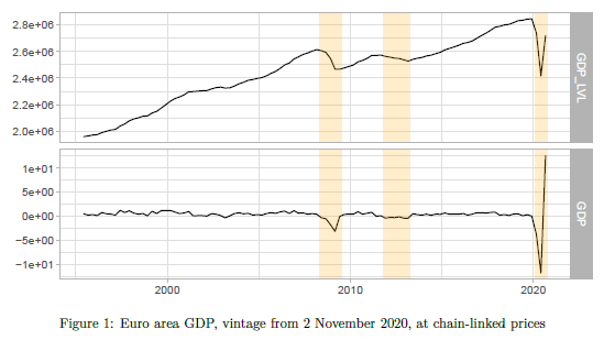
In this exercise, we use the data vintage downloaded from the ECB Statistical Data warehouse and the European Commission website on 2 November 2020. Our target variable is the euro area GDP at chain-linked prices. For our out-of-sample forecasting exercise of GDP growth we use the following auxiliary monthly time series: 1) euro area industrial production excluding construction, IIP; 2) intra-euro area exports of goods, EXI; 3) extra-euro area exports of goods, EXJ; 4) euro area industrial orders, IOR; 5) euro area Economic Sentiment Index, ESI. Consequently, there are four hard and one soft indicators. The soft indicator is characterised by a shorter publication lag than its hard counterparts. The hard indicators are the same as in Perez-Quiros et al. (2020).

The time series of the euro area GDP are shown in Figure 1. The level is displayed in the upper panel and the derived quarterly growth rate is displayed in the lower panel. The COVID-19 pandemic induced unprecedented swings in the GDP dynamics. The trough reached in the second quarter of 2020 is as low as the real GDP level observed in 2005. Naturally, this is reflected in the growth rates. In the first quarter of 2020 the estimated GDP growth rate was comparable to the worst drop in GDP during the Great Recession. In the second and third quarters of 2020, we observed an even more staggering fall and a subsequent rise in GDP of about 11.8 and 12.5 percentage points, respectively. The sample period from the first quarter of 1995 to the third quarter of 2020 includes the three recessionary periods – the Great Financial Crisis (GFC), the European Debt Crisis (EDC), and the COVID-19 pandemic (CVD) – shown in the figures by the shaded area.

Forecasting exercise

We utilise the dynamic factor model in spirit of Camacho and Perez-Quiros (2010) in order to forecast the quarterly growth rate of euro area GDP. Our benchmark forecasts are simple averages of the historically observed euro area GDP growth rates available each period, whereas the model forecast is made using the dynamic factor model. Hence the difference between the historical mean model (HMM) forecasts and those of the dynamic factor model (DFM) should reflect the informative content of the five monthly indicators for euro area GDP growth.

The sample used for out-of-sample forecast evaluation starts in 2006Q1 and extends until 2020Q3. Such a choice of the forecast evaluation sample conveniently contains the three recessionary periods and allows us to explore the asymmetries in the forecasting performance of the naï ve benchmark and more sophisticated econometric model during recessionary and expansionary periods.

For each target quarter, forecasts are made after its end, i.e. in the beginning of the first month of the next quarter. The choice of such forecast origin ensures that the maximum information for the targeted quarter can be extracted from the monthly auxiliary indicators, taken into account their publication schedule.

Results

We measure the nominal forecasting performance of the two models in terms of Mean Squared Forecast Error (MSFE). For comparing the forecasting performance of the DFM relative to the HMM we rely on the relative MSFE (rMSFE), which measures the relative improvement/deterioration in the nominal MSFE brought about by the DFM compared to the HMM recording.

We report the forecast accuracy measures firstly computed for the period containing the GFC and EDC but excluding the COVID pandemic (2006Q1 – 2019Q4) and secondly for the period including all the three recessionary periods (2006Q1 – 2020Q3). In doing so, we can single out the effect of the COVID period on the measures of forecast accuracy and see what difference it makes when compared to the forecast accuracy computed for the pre-COVID period.

The results of the forecasting exercise for the pre-COVID period are reported in Table 1. First consider the results for the full sample. As can be seen, the DFM produces much lower MSFE than that of the HMM, corresponding to the reduction of about 61%. At the first glance this suggests the obvious superiority of the more sophisticated model over the naïve benchmark.

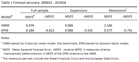
However, this first impression turns out to be misleading when we compare the forecasting performance of the models in question separately for expansions and recessions.

For expansions, it turns out that the DFM produces MSFE that is about 33% higher than that of the HMM, suggesting that during normal times it is safer to rely on the benchmark model forecasts. For recessions, however, the opposite is the case. The DFM model produces much lower MSFE than the HMM does. This is the expected result as by construction the HMM forecasts are totally backwards looking and therefore much less responsive to the large swings of GDP growth that typically take place during recessions.

When one compares the nominal values of the MSFE during expansions and recessions it becomes clear that the forecasting accuracy of the both models deteriorates during recessions, but for the HMM the deterioration is much more pronounced. Namely, this fact substantially contributes to the relative improvement of the forecasting accuracy of the DFM over the HMM during recessions. In fact, these relative gains during recessions turn out such large that they totally overshadow forecast losses accrued to the DFM during the expansionary period, further translating into the relative improvement reported for the whole sample.

A similar conclusion can be drawn when analysing the forecasting accuracy for the period including the COVID-19 pandemic, see Table 2.

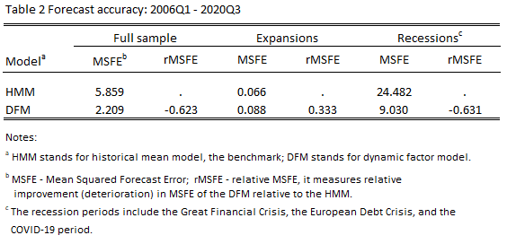
In Table 2 we see how adding observations for the COVID-19 pandemic drastically changed the forecast accuracy measures (MSFE) during recessions, naturally surfacing also in the MSFEs reported for the full sample. For the historical mean model the MSFE during recessions exceeds the one obtained during expansions by 24.482/0.066 = 370.9 times whereas for the DFM – by 9.030/0.088 = 102.6 times; a substantial difference from the corresponding MSFE ratios computed for the pre-COVID-19 period: 2.146/0.066 = 32.5 times – for the HMM and 0.577/0.088 = 6.6 times – for the DFM, see Table 1.

Summarising, one can say that recessions serve as bonanza for forecasters, by creating such a forecasting environment when few observations during volatile times may easily overturn the evidence based on many more observations during the relatively tranquil times. This tends to create the illusory superiority of the more sophisticated model over the benchmark model. In our example, if there were no recessions the DFM would not come under consideration for forecasting purposes.

The pandemic will eventually fade away but its effects in many areas will remain for years to come. The trade of forecasting is not an exception. In this note we illustrated how reliance on the standard forecast evaluation metric can lead to erroneous conclusions in case when the aberrant observations specifically during the COVID-19 pandemic and, more generally, during economic recessions are not properly taken into account. These biases can be avoided if one analyses and reports the forecasting performance of the competing models for expansions and recessions separately.