Using household-level data to guide borrower-based macro-prudential policy

Many countries introduced borrower-based instruments to constrain credit to households who exceed a certain limit on their loan-to-value ratio, on their (mortgage) debt-to-income ratio or on their debt service-to-income ratio. This paper evaluates how well borrower-based instruments can target those households that are financially vulnerable or would become vulnerable after a shock. We apply the signals approach to derive limits that are “optimal” in the sense of minimising classification errors (either granting credit to households that are financially vulnerable or constraining credit to households that are not financially vulnerable). We illustrate our methodology by simulating an adverse scenario using 2018 household-level data from Luxembourg. We find that combining several ratios could better target households that would become vulnerable after a shock.

1. Introduction

Since the global financial crisis, many developed countries have introduced borrower-based instruments allowing authorities to constrain the supply of credit for house purchase by setting an upper limit on various measures of a borrower’s debt burden. In the European Union, regular surveys by the European Systemic Risk Board (ESRB)3 show that most member states have been introducing limits on the loan-to-value ratio, fewer on the debt service-to-disposable income ratio or mortgage maturity, and even fewer on the debt-to-disposable income ratio.

In this paper, we perform an ex-ante evaluation of the effect of various borrower-based macro-prudential instruments on household financial vulnerability (Ampudia et al., 2016). Following Albacete et al. (2018) and Bańbula et al. (2016), we adapt the signals approach in Detken et al. (2014) to identify the settings of borrower-based instruments that most effectively target financially vulnerable households. Our study is innovative in considering combinations of several debt burden ratios with households being only credit constrained if they exceed several limits simultaneously. In addition, we explore an extension of the signals approach to account for household heterogeneity in terms of indebtedness and degree of financial vulnerability. Finally, our study illustrates how household-level data from surveys can help to set borrower-based instruments. Thus, it complements more aggregate approaches using macro-economic models4 or approaches based on bank data, which may contain less complete and less harmonized information about individual borrowers.

To empirically illustrate the methodology, we use data from the most recent wave of the Luxembourg Household Finance and Consumption Survey (LU-HFCS).

2. Data and debt burden ratios

The anonymous household-level data is drawn from wave 3 of the LU-HFCS conducted in 2018 with 1616 households. The sample was designed to be representative of the entire population of households resident in Luxembourg and is weighted accordingly. We focus on households that only recently took out their mortgage(s) on the household main residence (between 2015 and 2018), to better estimate the impact from activating borrower-based instruments.

Luxembourg authorities may impose limits on various ratios measuring a borrower’s debt burden, including the loan-to-value (LTV) ratio, the (mortgage) debt-to-disposable income ratio (MDI and DI), the debt service-to-disposable income ratio (DSI) or the mortgage maturity (MM). Only limits on the LTV ratio were activated in 2021, so we calculate how different values of LTV limits would have affected households with recent mortgages on their main residence, as well as the amount of credit that would not have been granted had the limits been in place in 2018.5

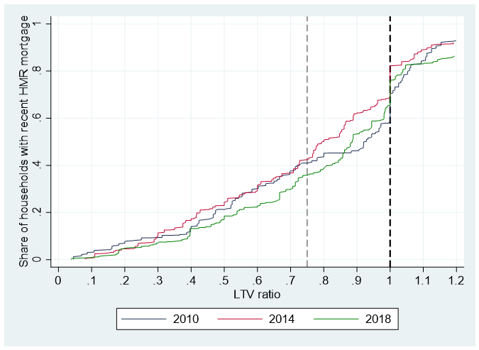
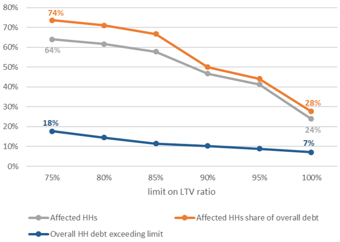
The least restrictive LTV limit envisaged by the law (100%) would have affected 24% of households with recent mortgages on their main residence (Figure 1). This would have required households with recent mortgages on their main residence to reduce their overall debt by 7% in order to comply with the limit. The most restrictive LTV limit envisaged by the law (75%) would have affected 64% of households with recent mortgages. This would have required them to reduce their overall debt by 18%. Some of the limits the law envisages for other ratios would have been even more restrictive (Giordana and Ziegelmeyer, 2022).

Figure 1: Initial loan-to-value (LTV) ratio
a) cumulative distribution by survey year

b) borrowers affected in 2018, their share of overall debt and the share of overall debt exceeding limit

Source: Own calculations based on waves 1, 2 and 3 of the LU-HFCS; data are multiply imputed and weighted; only households with recent HMR mortgages. Panel (a): cumulative distribution functions are calculated across all 5 implicates each year. Vertical lines indicate lowest and highest limits envisaged by the law. We omit the upper tail of the cumulative distribution functions.

3. Household financial vulnerability

Based on established practice, we measure a household financial vulnerability using an indicator of its probability of default and the bank’s loss given default associated with it. Following the literature6, we define household i’s probability of default (PDi) as a function of its monthly financial margin and its liquid asset holdings. The financial margin is measured as household gross income minus taxes, social security contributions, regular debt service payments and an estimate of basic living costs. A household’s probability of default is set to zero if it has a positive financial margin or if its liquid assets are sufficient to cover its negative financial margin for at least three months (matching the conventional 90-day limit used to define non-performing loans). Otherwise, the household’s probability of default is a simple function of its financial margin and its liquid assets. Thus, this indicator focuses on liquidity risk and measures the probability that the household falls behind in its debt payments.

The bank’s loss given default associated with household i (LGD_i) is the difference between the household’s total debt and real estate assets after applying a 25% haircut, weighted by the household probability of default.

As household defaults are not observed in our sample, the LGD measure should be understood as an expected amount. We classify a household as financially vulnerable if its LGD exceeds zero. A more conservative definition of financially vulnerable households only requires their PD to exceed zero. Table 1 reports the share of financially vulnerable households in 2018 using both definitions. The benign economic environment in 2018 suggests a very low share of households with a PD>0 or a LGD>0. However, even in such a favourable environment, macro-prudential instruments should focus on those households who may become financially stressed if economic conditions deteriorate.

Table 1: Share of households that become financially vulnerable in the adverse scenario compared to the 2018 baseline

Source: Giordana and Ziegelmeyer (2022). Calculations based on wave 3 of the LU-HFCS; data are multiply imputed and weighted.

Building on Giordana and Ziegelmeyer (2020), we simulate household balance sheets in an adverse economic scenario to identify which households are more vulnerable to financial stress. Our adverse economic scenario assumes a 12% unemployment rate. This is definitely a tail risk as it represents an extreme shock by Luxembourg standards, more than doubling the 2019 unemployment rate. We consider only one scenario to demonstrate how our proposed methodology works in practice. As expected, the share of vulnerable households increases substantially in the adverse scenario (Table 1). This is because the fall in labour income of unemployed individuals leads to a reduction of the household financial margin (other things equal), increasing both the probability of default and the loss given default.

4. Evaluating different policy rules

We implement a technique known as the “signals approach” (Kaminsky et al., 1998) or “signalling approach” (Detken et al., 2014) to identify policy settings that are “optimal” in the sense that they minimise classification errors.7 To compare classification rules, we use the Receiver Operating Characteristic (ROC) curve. In particular, the Area under the ROC curve (AUROC), a statistic ranging from 0 to 1, summarises the performance of each classification rule across all candidate limits. A classification rule with an AUROC of 1 is perfectly informative, while one with an AUROC of 0.5 is uninformative.8

There are two possible errors: type I classification errors correspond to “false positive” cases (households incorrectly classified as vulnerable), type II errors correspond to “false negative” cases (households incorrectly classified as not vulnerable). Varying the limit reveals a trade-off between these two types of classification errors. For instance, higher limits will reduce the number of households classified as vulnerable and therefore increase type II errors (missing some vulnerable households). Lower limits will raise the number of households classified as vulnerable and therefore increase type I errors (identifying too many households as vulnerable). Policymakers cannot avoid this trade-off in selecting their preferred setting. Thus, we minimise a loss function formulated as a linear combination of classification errors to find the “optimal” limit. Varying the loss function weight Ө allows us to consider different policy preferences regarding the trade-off between types of classification error.

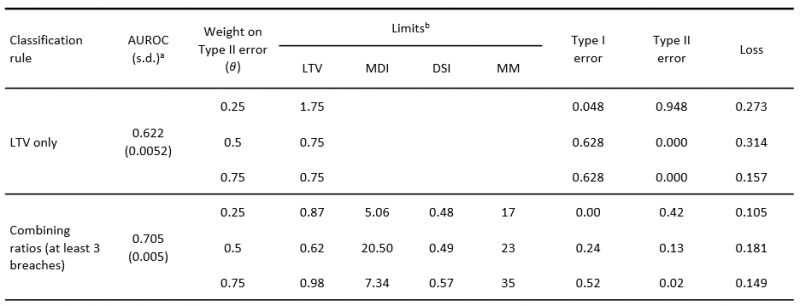
Table 2 evaluates how different classification rules perform at identifying households who were not vulnerable in the baseline but become financially vulnerable in the adverse scenario. The rule in the top row only considers the LTV ratio in isolation, while the rule in the second row combines different ratios but requires a household to breach at least three limits to be classified a financially vulnerable. While the AUROC is lower for the rule that only uses the LTV ratio, it is statistically higher than 0.5, confirming that the LTV ratio is informative to identify financial vulnerability. “Optimal” limits are within the legal range at Ө = 0.5 and Ө = 0.75. The rule combining different ratios achieves a higher AUROC and a lower Loss function.

Table 2: Performance of selected borrower-based measures in the adverse scenario

Source: Giordana and Ziegelmeyer (2022). Calculations based on the 3rd wave of the LU-HFCS; data are multiply imputed and weighted; the statistics are calculated by pooling all implicates. Notes: See Giordana and Ziegelmeyer (2022) for definitions of loan-to-value ratio (LTV), mortgage-debt-to-income ratio (MDI), debt-to-income ratio (DI), debt-service-to-income ratio (DSI), mortgage maturity (MM), type I and type II classification errors and Loss. ^a Standard deviation of Area Under the Receiver Operating Characteristic (AUROC) is based on Hanley and McNeil (1982). ^b Maximum legal limits are 1 for the LTV ratio, 12 for the MDI ratio, 0.75 for the DSI ratio and 35 years for MM.

The signals approach assigns the same weight to every household, regardless of its individual situation. This implicitly assumes that the cost of misclassification is the same across households, which tends to weaken the link between minimising classification errors and the policymaker objective of maximising social welfare. Since individual households carry different debt burdens, they may contribute differently to social costs and benefits, so we plot cost frontiers comparing the share of mortgage debt “incorrectly” granted to the share of debt “incorrectly” denied at different policy settings.

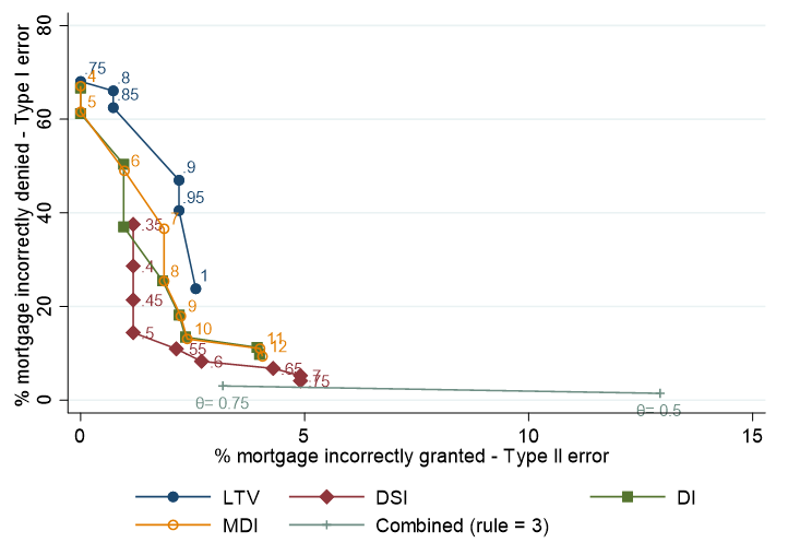
Figure 2 depicts the cost frontiers, which plot the share of total mortgage volume that would be incorrectly denied under the policy (type I error) against the share of total mortgage volume that would be granted incorrectly (type II error). The closer the cost frontier is to the origin, the smaller the costs of classification errors. For policy rules based on individual ratios, the markers indicate the outcomes for selected values of the limits within the legal range. For the policy rule combining different ratios, the markers show the outcome for different values of Ө. Limits on the DSI ratio clearly perform better than limits on the other individual ratios, as the associated frontier is closer to the origin. However, the policy combining ratios performs even better (with Ө = 0.75).

Figure 2: Cost frontiers – households with recent HMR mortgages (adverse scenario)

Source: Giordana and Ziegelmeyer (2022). Calculations based on the 3rd wave of the LU-HFCS; data are multiply imputed and weighted; classification errors are calculated by pooling all implicates.

5. Discussion and conclusion

This paper proposes a data-driven approach to guide borrower-based macro-prudential policy using data on individual households. By simulating an adverse scenario, we show that simultaneously considering several ratios would be more effective at identifying households who were not financially vulnerable in the benign conditions of 2018, but would become vulnerable after a severe income shock.

However, our results are subject to several caveats. First, we do not observe household defaults, since there is no functioning credit register in Luxembourg. Therefore, we use survey data to identify financially vulnerable households, which requires estimates of disposable income and basic living costs, and thus introduces some uncertainty in the results.

Second, our sample is limited to households who were actually granted mortgages, ignoring those who were refused credit and remained renters. Since households who rent have lower income, this may introduce a selection bias, possibly lowering our estimates of “optimal” policy settings. However, this bias should be negligible if the number of rejections is limited or if rejections are correlated with our measure of financial vulnerability, which seems likely. Moreover, our limited sample size increases the uncertainty around our point estimates, in particular for the “optimal” policy settings, which should be interpreted with this caveat.

Finally, we do not consider how private agents may respond either to the introduction of a borrower-based measure or to the negative income shock in the adverse economic scenario.

To conclude, our analysis finds that the “optimal” setting of borrower-based instruments will vary with the definition of household financial vulnerability, with policymaker preferences with respect to the trade-off between type I and type II errors, and with underlying economic conditions. Thus, our analysis provides a framework to assist in policy design by rendering explicit the definitions, assumptions and scenarios that need to be adjusted to reflect policymaker preferences or evolving economic conditions. Taking into consideration these limitations of the framework, our results can complement those from other analyses.

References

Albacete, N., and P. Fessler (2010): Stress Testing Austrian Households. Österreichische Nationalbank Financial Stability Report 19, June.
Albacete, N., Fessler, P., and P. Lindner (2018): One policy to rule them all? On the effectiveness of LTV, DTI and DSTI ratio limits as macroprudential policy tools. Financial Stability Report 35, Österreichische Nationalbank, June.
Ampudia, M., H. van Vlokhoven, and D. Zochowski (2016): Financial fragility of euro area households. Journal of Financial Stability, 27, 250–262.
Bańbuła, P., Kotuła, A., Przeworska J., and P. Strzelecki (2016): Which households are really financially distressed: How micro data could inform the macroprudential policy. IFC Bulletins chapters, Bank for International Settlements (eds.), Combining micro and macro statistical data for financial stability analysis, vol. 41, Basel.
Detken, C., Weeken, O., Alessi, L., Bonfim, D., Boucinha, M., Castro, C., Frontczak, S., Giordana, G., Giese, J., Jahn, N., Kakes, J., Klaus, B., Lang, J., Puzanova, N., and P. Welz (2014): Operationalising the countercyclical capital buffer: indicator selection, threshold identification and calibration options. ESRB Occasional Paper Series, 5, 1-95.
Giordana, G. and M. Ziegelmeyer (2020): Stress testing household balance sheets in Luxembourg. Quarterly Review of Finance and Economics, 76, 115-138. Previous version published as BCL Working Paper 121. July 2018.
Giordana, G., and M. Ziegelmeyer (2022): Using household level data to guide borrower-based macro-prudential policy. BCL working paper 161.
Hanley, J.A., and B. McNeil (1982): The meaning and use of the Area under a Receiver Operating Characteristic (ROC) Curve. Radiology, 143(1), 29-36.
Kaminsky, G., Lizondo, S., and C. Reinhart (1998): Leading indicators of currency crises. IMF Staff Papers, 45(1), 1–48.
Meriküll, J., and T. Rõõm (2020): Stress tests of the household sector using microdata from survey and administrative sources. International Journal of Central Banking, 16(2), 203-248.
Sangaré, I. (2019): Housing sector and optimal macro-prudential policy in an estimated DSGE model for Luxembourg. BCL Working Paper 129.
• 1.
Banque centrale du Luxembourg (BCL). E-mail: gaston_andres.giordana@bcl.lu
• 2.
Banque centrale du Luxembourg (BCL). E-mail: michael.ziegelmeyer@bcl.lu
• 3.
See https://www.esrb.europa.eu/national_policy/html/index.en.html.
• 4.
See Sangaré (2019) for a study based on a DSGE modelling approach applied to Luxembourg.
• 5.
Giordana and Ziegelmeyer (2022) discuss this for the other ratios as well.
• 6.
See Albacete and Fessler (2010); Ampudia et al. (2016); Giordana and Ziegelmeyer (2020); Meriküll and Rõõm (2020).
• 7.
This does not necessarily correspond to minimising the policymaker’s loss function, which would require specifying the links between classification errors, systemic risk and social welfare.
• 8.
For further explanations and relevant references, see Giordana and Ziegelmeyer (2022).
About the authors
Gastón Andrés Giordana
Gastón Andrés Giordana is a Senior Economist at the Research and Economics Department of the Central Bank of Luxembourg. He performs theoretical and empirical micro-economic analyses on various topics including individuals’ health expenditures and financial vulnerability, banking regulation, macro-prudential policy instruments, and virtual currencies.
Michael H. Ziegelmeyer
Michael Heinrich Ziegelmeyer is a Senior Economist at the Economics and Research Department of the Central Bank of Luxembourg following periods at the Monetary Policy Research Division at the ECB, the Mannheim Research Institute for the Economics of Aging, and Deutsche Bank Research. His research focuses on Household Finance. He received a PhD in Economics from the University of Mannheim in 2011 and teaches Household Finance at the University of Luxembourg.
More on these topics