Why do households save?

This paper examines whether the determinants of household saving have changed over time and whether they are the same across countries. Using a cross-country data for 34 OECD countries for the 1970-2019, we find that old saving rate specifications still perform strikingly well and can explain the recent changes in household saving rates. As for the cross-country differences in equilibrium saving rates, we have less success even though the basic estimating equations fit reasonably well to individual country samples. We found that household saving is still very sensitive to changes in real income growth and inflation. Thus, decline in the household saving rates after the 1980s can mainly be attributed to these variables. Obviously, a decline of real interest rate has also pushed down the saving rate. Moreover, households seem to have reacted to changes in public sector as well as corporate sector saving.

1. Introduction

Household saving is important for many reasons: it (1) provides information of future perception of consumption and income (in the sense of “saving for the rainy day”), (2) it determines future development of household indebtedness, (3) it provides information of the magnitude of debt neutrality; i.e. how much households pay attention to the developments of public debt (and higher taxes in the future), (4) its behavior indicates how much substitution there is between household and corporate savings that relevant for small businesses where the borderline between household and firm income is often unclear, (5) it provides information of the interest rate sensitivity of household behavior and, finally, (6) it provides information of life-cycle behavioral patterns of households.

That is why it is useful to revisit household saving function estimates to see whether the “old” behavioral relationship still works in the same way as earlier. It is also worth reconsidering the cross-country differences between countries to see the magnitude of these differences both from the data and after controlling the saving rate with an appropriate set of control variables.

In the past, there have been several cross-country analyses of which we might mention at the least the following: Callen and Thimann (1997) and Rocher and Stierle (2015). In addition, we may mention Edwards (1995) and Ferrucci and Mirales (2007) who focus on this question from the point of view of private saving. All afore mentioned studies use a similar panel data set-up with annual cross-country data with different choice of countries and sample periods. Here we use the maximum amount of household data from the OECD that cover the period 1970-2019. In addition to the household data, we also focus on the corporate sector saving (i.e. profits) and thereby private sector saving but because the results for the latter are qualitatively almost identical we concentrate here on household saving.

2. Analysis

The empirical analysis is carried out in a customary way by estimating a saving rate equation from a cross-country panel data consisting of 34 countries and covering the time period 1970-2019. The estimating equation for the saving rate takes the following form:

sr = α₀ + α₁s_-1 + α₂yd + α₃π + α₄rr +control variables + μ_t

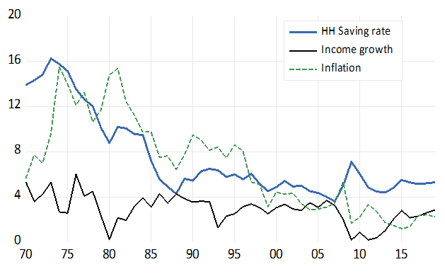
where sr is the saving rate, yd household real (disposable) income growth, π inflation and rr the real (long-term) interest rate and μ the error term. The model is basically an extended version of the old Deaton (1977) model where the driving force is inflation reflecting consumers’ inability to distinguish individual commodity price increases from overall inflation. If prices increase, people experience these increases as increases on relative prices of goods that they are sampling. Thus, they reduce the demand for these goods and that leads first to a fall in aggregate consumption demand, which in turn translates to an increase in the saving rate. It follows, that in the saving rate equation, real income growth and inflation are the key variables. The country mean values of these variables are displayed in Figure 1. Real interest rate is added just to take account of the slope of the consumption growth locus. As for the controls, we comment on their role below. The equation is estimated by both OLS and Arellano-Bond GMM using different panel-data set-ups. The details of the data and estimation are explained in Oinonen and Viren (2019).

Figure 1. Cross-country mean values of the saving rate, income growth and inflation

The main results are reported in Table 1. Besides estimating the basic equation we estimated a static version of that in order to see how well we can explain the levels of country differences. Thus, we dropped the lagged value of saving rate s_r-1, household indebtedness, income growth and inflation from the estimating equation, which then only included the control variables on the right-hand-side. The respective results revealed that we cannot really account for most of household saving rate differences across countries. It is only if we introduce country fixed effects, R² increased to 0.85. With the fixed time effects R² is 0.49 and without all fixed effects 0.44. Most of the controls were statistically significant, but even then, the levels of saving seem to depend on some third (more complex institutional or cultural) variables.

Given this somewhat disappointing (even though old) result we turn to results with the dynamic specification. In a dynamic version, the explanatory power is reasonable, particularly when we introduce the fixed country and period effects. The controls do increase the explanatory power but do not really change the key ingredients of the basic specification. Thus, we observe that the household saving rate depends very strongly (and positively) on disposable income growth, inflation and real interest rate. In fact, these results also apply to the private saving rate (column 3).

The basic equation performs strikingly well also if we estimate the coefficients for individual countries separately. Thus, for α₁, all coefficients are positive, for α₂ one (country) coefficient is negative, for α₃ and α₄ four coefficients (out of 34) are negative. The basic model (without controls) performs very well and is very robust in terms of sample selection and estimation method (OLS vs. GMM). When controls are introduced, the signs, significance and magnitude of the key variables do not change. It is only that some of the controls are sensitive to the estimation method. Thus, if we use the GMM with first differences, variables like GDP per capita and the gross tax rate change the sign.

Table 1. Basic estimation results with the saving rate equation

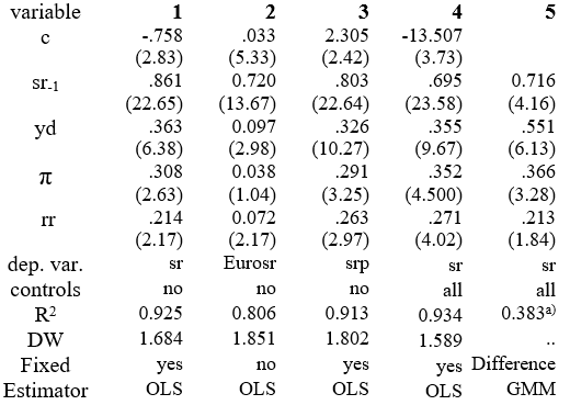
^a) Instead of the R² we have here the P value of the J statistic. sr (srp) denotes the household (private) saving rate. Eurosr is the household saving rate for the Euro area. With srp, the income growth variable is the growth rate of real private disposable income ydp. “Yes” on the “Fixed” line indicates inclusion of country and time fixed effects. Numbers inside parentheses are robust t-ratios. The number of data points with the basic model is 742 and with the model with all controls 613.

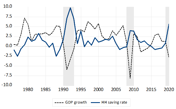
The positive association between real income growth and the saving rate means that consumption growth is much smoother than income growth because hikes in income are observed by additional savings. Inflation works to the same direction (to the extent inflation depends on cyclical factors) also smoothing consumption. To some extent, consumption smoothing seems to be nonlinear. Thus, if we focus on the coefficient α₂ for positive and negative values of real disposable income growth yd we find that the coefficient is seemingly very different as the following coefficient estimates indicate: α₂^– (which indicates the coefficient of yd|yd<0) = 0.261(with the t-value 1.65) and α₂⁺ (for yd|yd=>0) = 0.396(6.92). This suggests that positive and negative change rates of income affect saving differently. Thus, negative income shocks do not necessarily lower the saving rate but may even increase it due to the precautionary motive as a response to increased uncertainty; a conclusion that is consistent with recent experiences of the financial crisis and the Covid-19 pandemic (see Figure 2 for Finnish evidence)2. In fact, also inflation – and even the real interest rate have a nonlinear effect on the saving rate so that the coefficients for negative rates for inflation and real rates are not significant while positive values have a strong positive effect on saving.

So, we can say that savings respond disproportionally more to positive values of real income growth and inflation. Because of this nonlinearity, the saving rate channel provides only a partial “automatic stabilizer” for the economy. Big negative shocks are almost always associated with increase in uncertainty and that leads to increase in precautionary saving and fall in private consumption which may further aggravate the cyclical situation.

Although we find the coefficients of the saving rate equation are sensitive to the values of the regressors, we find that the coefficients are strikingly robust in terms of time. Thus, the estimates for pre and post Lehman are, if not identical, very similar to the full sample period counterparts. So, the sensitivity of saving with respect to inflation and interest rate have not diminished during the period of very low inflation and interest rates.

Figure 2. Cyclical behavior of the Finnish Saving rate

As for the controls we can conclude that

• the terms of trade tends to always increase saving; an increase in the terms of trade obviously means higher level of income in the country in question compared with other countries.
• the “deepness of credit markets” increases saving; this is something which is consistent with early findings of e.g. Goldsmith (1969) and McKinnon (1973).
• the share of public sector – measured as the share of public consumption out of GDP has an ambiguous effect. Ambiguity might arise from the fact that a part of public consumption is a substitute to private consumption. On the other hand, an increase in the size of government can be interpreted as an indication of higher taxes in the future.
• public sector surplus always decreases household saving which could be an indication of debt neutrality; households acknowledge that they must be prepared to smaller (higher) income (taxes) in the future
• household indebtedness increases household saving (as some sort of error-correction mechanism) but the size of the effect depends on other controls.
• the level of income per capita has a positive effect on saving.
• population growth increases saving along the lines of the “Modigliani story of aggregation”. According to this hypothesis, aggregative saving can be positive even though individual life-time saving is zero because in a growing economy there are more savers than dis-savers with a typical life-time profile where saving precedes dis-saving.
• self-employment has typically a positive effect on saving (due to more risky income).
• corporate sector profits have a negative effect on household saving, which is consistent with the old “saving substitution” story, in which the borderline between household and company saving is vague for at least small businesses.
• the gross tax-rate has a negative effect on saving – the explanation may be in the increase in tax progressivity which ultimately follows from higher over-all tax rates, which leads to lower disposable income of high savers and more equal income distribution.
• the effect of ageing is quite weak probably reflecting the fact that the profile of the age-dependency ratio in all countries is U -shaped due to high birth rates in the later 1940s and 1950s.

We also estimated equation (1) for the Euro Area using quarterly ECB data for 1995Q1-2019Q4. Again, the results followed the same lines as with the global cross-country panel (Table 1, column 2). The estimates again corroborates the predictions of Deaton (1977) even though inflation in the Euro Area has been almost constant for this sample period (the standard deviation of the 4-quarter growth rate is only 0.8 per cent while the mean being 1.6 per cent).

3. Conclusions

We have found that household saving is still very sensitive to changes in real income growth, inflation, and real interest rates. Thus, decline in the household saving rate after the 1990s can mainly be attributed to these variables. Households seem to react in a “correct way” to changes in public sector as well as corporate sector saving so that there is some degree of saving substitutability which could have partly compensated the developments of inflation and interest rates. The study also finds that cross-country differences in “equilibrium” saving rates are very large and cannot fully be explained by a conventional set of control variables.